
2019 ATB
For each electricity generation technology in the ATB, this website provides:
- Capital expenditures (CAPEX): the definition of CAPEX used in the ATB and the historical trends, current estimates, and future projections of CAPEX used in the ATB
- Operations and maintenance (O&M) costs: the definition of O&M and the current estimates and future projections of O&M used in the ATB
- Capacity factor (CF): the definition of CF and the historical trends, current estimates, and future projections of CF used in the ATB
- Future cost and performance methods: an outline of the methodology used to make the projections of future cost and performance in the ATB for Constant, Mid, and Low technology cost cases
- Levelized cost of energy (LCOE): metric that combines CAPEX, O&M, CF, and projections for Constant, Mid, and Low technology cost cases for illustration of the combined effect of the primary cost and performance components and discussion of technology advances that yield future projections
- Financing assumptions: development of technology-specific interest rate on debt, return on equity, and debt-to-equity ratios and their impact on LCOE are documented in each technology section, where applicable, and summarized here.
Electricity generation technologies are selected on the left side of the screen, and the topics highlighted above can be selected using the drop-down menu at the top right of the screen.
Guidelines for using and interpreting ATB content and comparisons to other literature are provided. LCOE accounts for many variables important to determining the competitiveness of building and operating a specific technology (e.g., upfront capital costs, capacity factor, and cost of financing); however, it does not necessarily demonstrate which technology in a given place and time would provide the lowest cost option for the electricity grid. Such analysis is performed using electric sector models such as the Regional Energy Deployment Systems (ReEDS) model and corresponding analysis results such as the NREL Standard Scenarios.
The NREL Standard Scenarios, a companion product to the ATB, provides a suite of electric sector scenarios and associated assumptions, including technology cost and performance assumptions from the ATB.
ATB data sources and references are also provided for each technology. All dollar values are presented in 2017 U.S. dollars, unless noted otherwise.
Additional information is available here: About the 2019 ATB.
Residential PV Systems
Representative Technology
For the ATB, residential PV systems are modeled for a 5.0-kWDC fixed tilt (25°), roof-mounted system. Flat-plate PV can take advantage of direct and indirect insolation, so PV modules need not directly face and track incident radiation. This gives PV systems a broad geographical application, especially for residential PV systems.
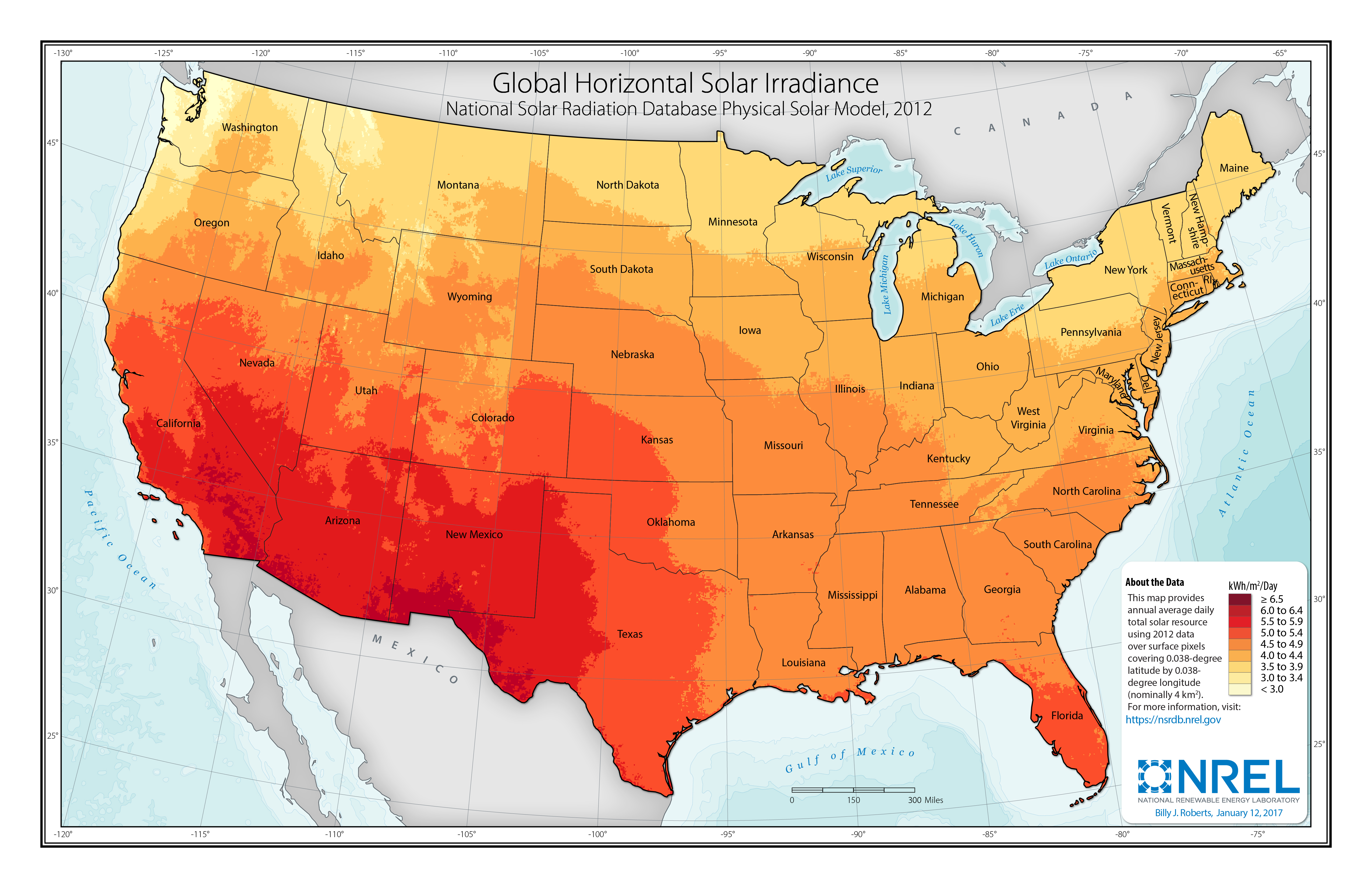
Resource Potential
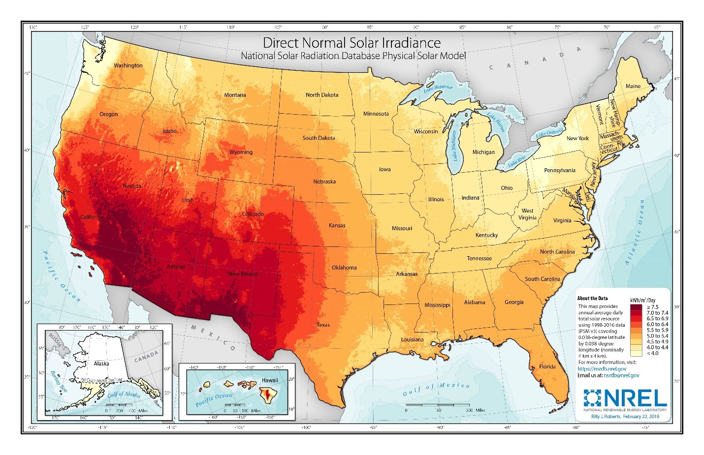
Solar resources across the United States are mostly good to excellent at about 1,000-2,500 kWh/m2/year. The Southwest is at the top of this range, while only Alaska and part of Washington are at the low end. The range for the contiguous United States is about 1,350-2,500 kWh/m2/year. Nationwide, solar resource levels vary by about a factor of two.
Distributed-scale PV is assumed to be configured as a fixed-tilt, roof-mounted system. Compared to utility-scale PV, this reduces both the potential capacity factor and amount of land (roof space) that is available for development. A recent study of rooftop PV technical potential (Gagnon et al. 2016) estimated that as much as 731 GW (926 TWh/yr) of potential exists for small buildings (< 5,000 m2) and 386 GW (506 TWh/yr) of potential exists for medium (5,000-25,000 m2) and large buildings (> 25,000 m2).
Renewable energy technical potential, as defined by Lopez et al. (2012), represents the achievable energy generation of a particular technology given system performance, topographic limitations, and environmental and land-use constraints. The primary benefit of assessing technical potential is that it establishes an upper-boundary estimate of development potential. It is important to understand that there are multiple types of potential-resource, technical, economic, and market (see NREL: "Renewable Energy Technical Potential").
Base Year and Future Year Projections Overview
The Base Year estimates rely on modeled CAPEX and O&M estimates benchmarked with industry and historical data. Capacity factor is estimated based on hours of sunlight at latitude for five representative geographic locations in the United States.
Future year projections are derived from analysis of published projections of PV CAPEX and bottom-up engineering analysis of O&M costs. Three different technology cost scenarios were developed for scenario modeling as bounding levels:
- Constant Technology Cost Scenario: no change in CAPEX, O&M, or capacity factor from 2017 to 2050; consistent across all renewable energy technologies in the ATB
- Mid Technology Cost Scenario: based on the median of literature projections of future CAPEX; O&M technology pathway analysis
- Low Technology Cost Scenario: based on the low bound of literature projections of future CAPEX and O&M technology pathway analysis.
Capital Expenditures (CAPEX): Historical Trends, Current Estimates, and Future Projections
Capital expenditures (CAPEX) are expenditures required to achieve commercial operation in a given year. These expenditures include the hardware, the balance of system (e.g., site preparation, installation, and electrical infrastructure), and financial costs (e.g., development costs, onsite electrical equipment, and interest during construction) and are detailed in CAPEX Definition. In the ATB, CAPEX reflects typical plants and does not include differences in regional costs associated with labor, materials, taxes, or system requirements. The related Standard Scenarios product uses Regional CAPEX Adjustments. The range of CAPEX demonstrates variation with resource in the contiguous United States.
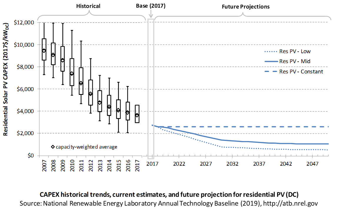
The following figure shows the Base Year estimate and future year projections for CAPEX costs. Three cost scenarios are represented: Constant, Mid, and Low technology cost. Historical data from residential PV installed in the United States are shown for comparison to the ATB Base Year estimates. The estimate for a given year represents CAPEX of a new plant that reaches commercial operation in that year.
Recent Trends
Reported residential PV installation CAPEX (Barbose and Dargouth 2018) is shown in box-and-whiskers format for comparison to historical residential PV benchmark overnight capital cost (Fu, Feldman, and Margolis 2018) and the ATB estimates of future CAPEX projections. The data in Barbose and Dargouth (2018) represent 81% of all U.S. residential and commercial PV capacity installed through 2016 and 75% of capacity installed in 2017.
The difference in each year's price between the market and benchmark data reflects differences in methodologies. There are a variety of reasons reported and benchmark prices can differ, as enumerated by Barbose and Dargouth (2018) and Bolinger and Seel (2018), including:
- Timing-related issues: For instance, the time between contract completion date and project placed in service may vary.
- Variations over time in the size, technology, installer margin, and design of systems installed in a given year
- Which cost categories are included in CAPEX (e.g., financing costs and initial O&M expenses).
Due to the investment tax credit, projects are encouraged to include as many costs incurred in the upfront CAPEX to receive a higher tax credit, which may have otherwise been reported as operating costs. The bottom-up benchmarks are more reflective of an overnight capital cost, which is in line with the ATB methodology of inputting overnight capital cost and calculating construction financing to derive CAPEX.
PV pricing and capacities are quoted in kWDC (i.e., module rated capacity) unlike other generation technologies, which are quoted in kWAC. For PV, this would correspond to the combined rated capacity of all inverters. This is done because kWDC is the unit that the majority of the PV industry uses. Although costs are reported in kWDC, the total CAPEX includes the cost of the inverter, which has a capacity measured in kWAC.
CAPEX estimates for 2018 reflect a continued rapid decline in pricing supported by analysis of recent system cost and pricing for projects that became operational in 2018 (Feldman and Margolis 2018).
Base Year Estimates
For illustration in the ATB, a representative residential-scale PV installation is shown. Although the PV technologies vary, typical installation costs are represented with a single estimate because the CAPEX does not vary with solar resource.
Although the technology market share may shift over time with new developments, the typical installation cost is represented with the projections above.
A system price of $2.77/WDC in 2017 and $2.64/WDC in 2018 are based on bottom-up benchmark analysis reported in U.S. Solar Photovoltaic System Cost Benchmark Q1 2018 (adjusted for inflation) (Fu, Feldman, and Margolis 2018). These figures are in line with other estimated system prices reported in Q2/Q3 2018 Solar Industry Update (Feldman and Margolis 2018).
The Base Year CAPEX estimates should tend toward the low end of observed cost because no regional impacts are included. These effects are represented in the historical market data.
Future Year Projections
Projections of future residential PV installation CAPEX are based on seven system price projections from six separate institutions made in the last two years. We adjusted the "min," "median," and "max" projections in a few different ways. All 2017 and 2018 pricing are based on the bottom-up benchmark analysis reported in U.S. Solar Photovoltaic System Cost Benchmark Q1 2018 (adjusted for inflation) (Fu, Feldman, and Margolis 2018). These figures are in line with other estimated system prices reported in Q2/Q3 2018 Solar Industry Update (Feldman and Margolis 2018).
We adjusted the Mid and Low cost projections for 2019-2050 to remove distortions caused by the combination of forecasts with different time horizons and based on internal judgment of price trends. The Constant technology cost scenario is kept constant at the 2018 CAPEX value, assuming no improvements beyond 2018.
A detailed description of the methodology for developing future year projections is found in Projections Methodology.
Technology innovations that could impact future O&M costs are summarized in LCOE Projections.
CAPEX Definition
Capital expenditures (CAPEX) are expenditures required to achieve commercial operation in a given year. For residential PV, this is modeled for a host-owned business model only.
For the ATB, and based on EIA (2016b) and the NREL Solar-PV Cost Model (Fu, Feldman, and Margolis 2018), the distributed residential solar PV plant envelope is defined to include:
- Hardware
- Module supply
- Power electronics, including inverters
- Racking
- Foundation
- AC and DC wiring materials and installation
- Balance of system (BOS)
- Site and/or roof preparation
- Permitting, inspection, and interconnection costs
- Project indirect costs, including costs related to engineering, distributable labor and materials, construction management start up and commissioning, and contractor overhead costs, fees, and profit
- Financial costs
- Owners costs, such as development costs, legal fees, insurance costs.
CAPEX can be determined for a plant in a specific geographic location as follows:
Regional cost variations are not included in the ATB (CapRegMult = 1). Because distributed PV plants are located directly at the end use, there are no grid connection costs (GCC = 0). In the ATB, the input value is overnight capital cost (OCC) and details to calculate interest during construction (ConFinFactor).
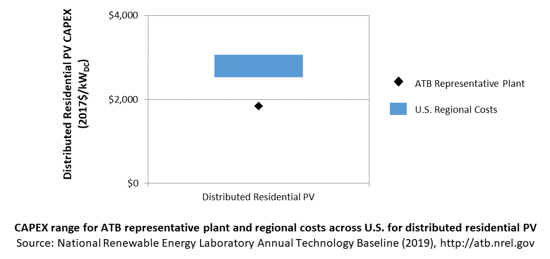
In the ATB, CAPEX represents a typical distributed residential/commercial PV plant and does not vary with resource. Regional cost effects associated with labor rates, material costs, and other regional effects as defined by EIA (2016b) expand the range of CAPEX. Unique land-based spur line costs based on distance and transmission line costs are not estimated. The following figure illustrates the ATB representative plant relative to the range of CAPEX including regional costs across the contiguous United States. The ATB representative plants are associated with a regional multiplier of 1.0.
Standard Scenarios Model Results
ATB CAPEX, O&M, and capacity factor assumptions for the Base Year and future projections through 2050 for Constant, Mid, and Low technology cost scenarios are used to develop the NREL Standard Scenarios using the ReEDS model. See ATB and Standard Scenarios.
CAPEX in the ATB does not represent regional variants (CapRegMult) associated with labor rates, material costs, etc., but dSolar does include 134 regional multipliers (EIA 2016b).
Operation and Maintenance (O&M) Costs
Operations and maintenance (O&M) costs represent the annual expenditures required to operate and maintain a solar PV plant over its lifetime, including:
- Insurance, property taxes, site security, legal and administrative fees, and other fixed costs
- Present value and annualized large component replacement costs over technical life (e.g., inverters at 15 years)
- Scheduled and unscheduled maintenance of solar PV plants, transformers, etc. over the technical lifetime of the plant (e.g., general maintenance, including cleaning and vegetation removal).
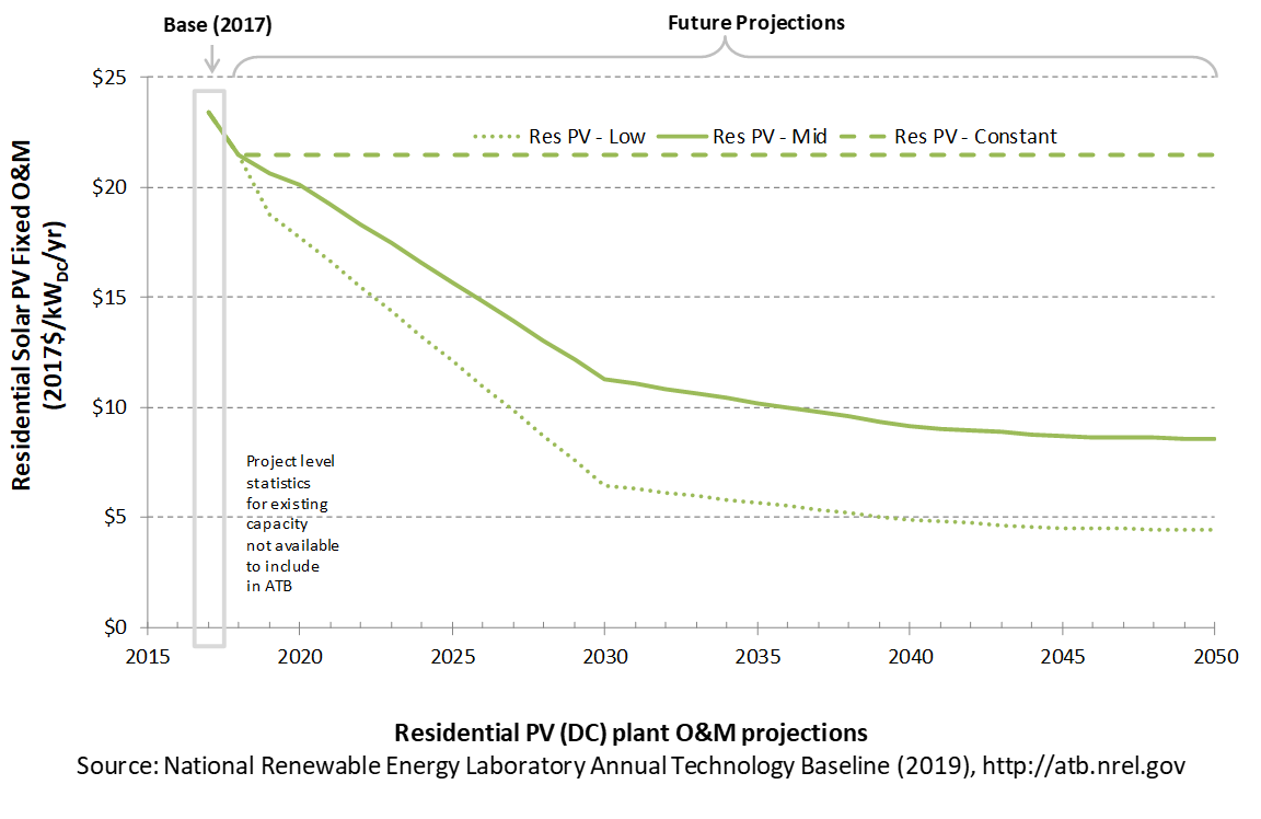
The following figure shows the Base Year estimate and future year projections for fixed O&M (FOM) costs. Three cost scenarios are represented. The estimate for a given year represents annual average FOM costs expected over the technical lifetime of a new plant that reaches commercial operation in that year.
Base Year Estimates
FOM of $23/kWDC - yr based on modeled pricing for a commercial PV system quoted in Q1 2017 as reported by Fu, Feldman, and Margolis (2018), adjusted for inflation. The values in this report (ATB 2019) are higher than those from ATB 2018 to better align with the benchmarks reported in Fu, Feldman, and Margolis (2018); the previous edition relied solely on an O&M-to-CAPEX ratio, derived from multiple reports. A wide range in reported prices exists in the market, and in part, it depends on what maintenance practices exist for a particular system. These cost categories include asset management (including compliance and reporting for incentive payments), different insurance products, site security, cleaning, vegetation removal, and failure of components. Not all these practices are performed for each system; additionally, some factors depend on the quality of the parts and construction. NREL analysts estimate O&M costs can range from $0 to $40/kWDC - yr.
Future Year Projections
FOM for 2018 is also based on pricing reported in Fu, Feldman, and Margolis (2018), adjusted for inflation. From 2019-2050, FOM is based on the historical average ratio of O&M costs ($/kW-yr) to CAPEX costs ($/kW), 0.8:100, as reported by Fu, Feldman, and Margolis (2018). Historically reported data suggest O&M and CAPEX cost reductions are correlated; from 2010 to 2018 benchmark residential PV O&M and CAPEX costs fell 60% and 63% respectively, as reported by Fu, Feldman, and Margolis (2018).
A detailed description of the methodology for developing future year projections is found in Projections Methodology.
Technology innovations that could impact future O&M costs are summarized in LCOE Projections.
Capacity Factor: Expected Annual Average Energy Production Over Lifetime
The capacity factor represents the expected annual average energy production divided by the annual energy production, assuming the plant operates at rated capacity for every hour of the year. It is intended to represent a long-term average over the lifetime of the plant. It does not represent interannual variation in energy production. Future year estimates represent the estimated annual average capacity factor over the technical lifetime of a new plant installed in a given year.
PV system capacity is not directly comparable to other technologies' capacity factors. Other technologies' capacity factors are represented in exclusively AC units (see Solar PV AC-DC Translation). However, because PV pricing in this ATB documentation is represented in $/WDC, PV system capacity is a DC rating. Because each technology uses consistent capacity ratings, the LCOEs are comparable.
The capacity factor is influenced by the hourly solar profile, technology (e.g., thin-film versus crystalline silicon), axis type (e.g., none, one, or two), expected downtime, and inverter losses to transform from DC to AC power. The DC-to-AC ratio is a design choice that influences the capacity factor. PV plant capacity factor incorporates an assumed degradation rate of 0.75%/year (Fu, Feldman, and Margolis 2018) in the annual average calculation. R&D could lower degradation rates of PV plant capacity factor; future projections for Mid and Low cost scenarios reduce degradation rates by 2050, using a straight-line basis, to 0.5%/year and 0.2%/year respectively.
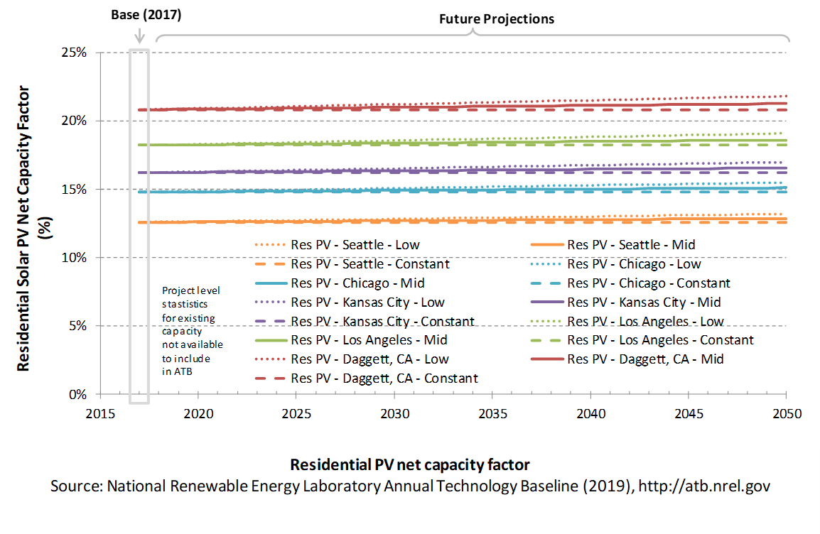
The following figure shows a range of capacity factors based on variation in solar resource in the contiguous United States. The range of the Base Year estimates illustrate the effect of locating a utility-scale PV plant in places with lower or higher solar irradiance. These five values use specific locations as examples of high (Daggett, CA), high-mid (Los Angeles, CA), mid (Kansas City, MO), low-mid (Chicago, IL), and low (Seattle, WA) resource areas in the United States as implemented in the System Advisor Model using PV system characteristics from Fu, Feldman, and Margolis (2018).
Base Year Estimates
For illustration in the ATB, a range of capacity factors is associated with the range of solar irradiance for three resource locations in the contiguous United States:
- Low: Seattle, Washington
- Low-mid: Chicago, Illinois
- Mid: Kansas City, Missouri
- High-mid: Los Angeles, California
- High: Daggett, California
First-year operation capacity factors as modeled range from 13.4% to 22.2%, though these depend significantly on geography and system configuration (e.g., fixed-tilt versus single-axis tracking).
Over time, PV installation output is reduced due to degradation in module quality. This degradation is accounted in ATB estimates of capacity factor over the 30-year lifetime of the plant. The adjusted average capacity factor values in the ATB Base Year are 12.6%, 14.8%, 16.2%, 18.2%, and 20.8%.
Future Year Projections
Projections of capacity factors for plants installed in future years are unchanged from the Base Year for the Constant technology cost scenario. Capacity factors for Mid and Low cost scenarios are projected to increase over time, caused by a straight-line reduction in PV plant capacity degradation rates, reaching 0.5%/year and 0.2%/year by 2050 for the Mid and Low cost scenarios respectively. The following table summarizes the difference in average capacity factor in 2050 caused by different degradation rates in the Constant, Mid, and Low cost scenarios.
| Seattle, WA | Chicago, IL | Kansas City, MO | Los Angeles, CA | Daggett, CA | |
| Low Cost (0.30% degradation rate) | 13.1% | 15.4% | 16.8% | 18.9% | 21.6%< |
| Mid Cost (0.50% degradation rate) | 12.9% | 15.1% | 16.6% | 18.6% | 21.3% |
| Constant Cost (0.75% degradation rate) | 12.6% | 14.8% | 16.2% | 18.2% | 20.8% |
Solar PV plants have very little downtime, inverter efficiency is already optimized, and tracking is already assumed. That said, there is potential for future increases in capacity factors through technological improvements beyond lower degradation rates, such as less panel reflectivity and improved performance in low-light conditions.
Standard Scenarios Model Results
ATB CAPEX, O&M, and capacity factor assumptions for the Base Year and future projections through 2050 for Constant, Mid, and Low technology cost scenarios are used to develop the NREL Standard Scenarios using the ReEDS model. See ATB and Standard Scenarios.
dSolar does not endogenously consider curtailment from surplus renewable energy generation, though this is a feature of the linked ReEDS-dSolar model (Cole et al. 2016), where balancing area-level marginal curtailments can be applied to distributed PV generation as determined by scenario constraints.
Plant Cost and Performance Projections Methodology
Currently, CAPEX – not LCOE – is the most common metric for PV cost. Due to differing assumptions in long-term incentives, system location and production characteristics, and cost of capital, LCOE can be confusing and often incomparable between differing estimates. While CAPEX also has many assumptions and interpretations, it involves fewer variables to manage. Therefore, PV projections in the ATB are driven entirely by plant and operational cost improvements.
We created Constant, Mid, and Low technology cost CAPEX cases to explore the range of possible outcomes of future PV cost improvements. The Constant technology case represents no CAPEX improvements made beyond today, the Mid case represents current expectations of price reductions in a "business-as-usual" scenario, and the Low case represents current expectations of potential cost reductions given improved R&D funding and more aggressive global deployment targets.
While CAPEX is one of the drivers to lower costs, R&D efforts continue to focus on other areas to lower the cost of energy from residential PV. While these are not incorporated in the ATB, they include longer system lifetime, improved performance and reliability, and lower cost of capital.
Projections of future residential PV installation CAPEX are based on seven system price projections from six separate institutions. Projections include short-term U.S. price forecasts and long-term global and U.S. price forecasts made in the past two years. The short-term forecasts were primarily provided by market analysis firms with expertise in the PV industry, through a subscription service with NREL. The long-term forecasts primarily represent the collection of publicly available, unique forecasts with either a long-term perspective of solar trends or through capacity expansion models with assumed learning by doing.
- Short-Term Forecast Institutions: Bloomberg New Energy Finance, CAISO, GTM Research, Navigant Research (Labastida and Gauntlett 2016), U.S. Energy Information Administration
- Long-Term Forecast Institutions: Bloomberg New Energy Finance, International Energy Agency.
In instances in which literature projections did not include all years, a straight-line change in price was assumed between any two projected values. To generate Mid and Low technology cost scenarios we took the "median" and "min" of the data sets; however, we only included short-term U.S. forecasts until 2030 as they focus on near-term pricing trends within the industry. Starting in 2030, we include long-term global and U.S. forecasts in the data set, as they focus more on long-term trends within the industry. It is also assumed after 2025 U.S. prices will be on par with global averages. Many of the global projections are weighted heavily toward western countries (e.g., European countries, Japan, and the United States), and in the long-term, the United States should follow global trends. The federal tax credit for solar assets reverts down to 10% for all projects placed in service after 2023, which has the potential to lower upfront financing costs and remove any distortions in reported pricing, compared to other global markets. Additionally, a larger portion of the United States will have a more mature PV market, which should result in a narrower price range. Many institutions used one system price for all countries. Changes in price for the Mid and Low technology cost scenarios between 2020 and 2030 are interpolated on a straight-line basis.
We adjusted the "median" and "min" projections in a few different ways. All 2017 and 2018 pricing are based on the bottom-up benchmark analysis reported in U.S. Solar Photovoltaic System Cost Benchmark Q1 2018 (adjusted for inflation) (Fu, Feldman, and Margolis 2018). These figures are in line with other estimated system prices reported in Q2/Q3 2018 Solar Industry Update (Feldman and Margolis 2018).
We adjusted the Mid and Low cost projections for 2019-2050 to remove distortions caused by the combination of forecasts with different time horizons and based on internal judgment of price trends. The Constant technology cost scenario is kept constant at the 2018 CAPEX value, assuming no improvements beyond 2018.

From 2019-2050, FOM is based on the historical average ratio of O&M costs ($/kW-yr) to CAPEX costs ($/kW), 0.8:100, as reported by Fu, Feldman, and Margolis (2018). Historically reported data suggest O&M and CAPEX cost reductions are correlated; from 2010 to 2018 benchmark residential PV O&M and CAPEX costs fell 60% and 63% respectively, as reported by Fu, Feldman, and Margolis (2018).
Projections of capacity factors for plants installed in future years are unchanged from 2018 for the Constant technology cost scenario. Capacity factors for Mid and Low cost scenarios are projected to increase over time, caused by a straight-line reduction in PV plant capacity degradation rates from 0.75%, reaching 0.5%/year and 0.2%/year by 2050 for the Mid and Low cost scenarios, respectively.
Levelized Cost of Energy (LCOE) Projections
Levelized cost of energy (LCOE) is a summary metric that combines the primary technology cost and performance parameters: CAPEX, O&M, and capacity factor. It is included in the ATB for illustrative purposes. The ATB focuses on defining the primary cost and performance parameters for use in electric sector modeling or other analysis where more sophisticated comparisons among technologies are made. The LCOE accounts for the energy component of electric system planning and operation. The LCOE uses an annual average capacity factor when spreading costs over the anticipated energy generation. This annual capacity factor ignores specific operating behavior such as ramping, start-up, and shutdown that could be relevant for more detailed evaluations of generator cost and value. Electricity generation technologies have different capabilities to provide such services. For example, wind and PV are primarily energy service providers, while the other electricity generation technologies provide capacity and flexibility services in addition to energy. These capacity and flexibility services are difficult to value and depend strongly on the system in which a new generation plant is introduced. These services are represented in electric sector models such as the ReEDS model and corresponding analysis results such as the Standard Scenarios.
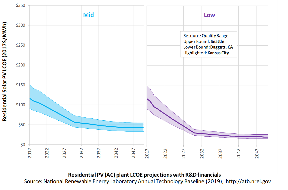
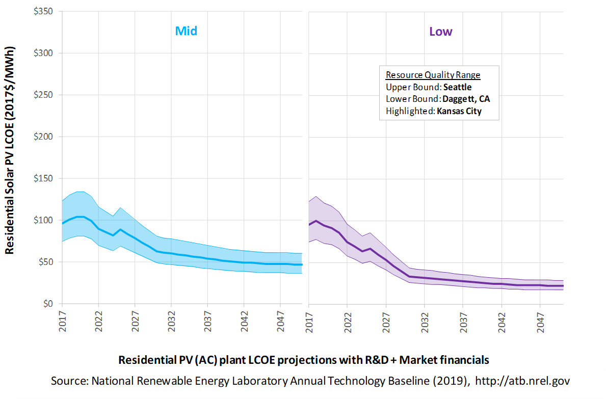
The following three figures illustrate LCOE, which includes the combined impact of CAPEX, O&M, and capacity factor projections for residential PV across the range of resources present in the contiguous United States. For the purposes of the ATB, the costs associated with technology and project risk in the U.S. market are represented in the financing costs but not in the upfront capital costs (e.g., developer fees and contingencies). An individual technology may receive more favorable financing terms outside of the United States, due to less technology and project risk, caused by more project development experience (e.g., offshore wind in Europe) or more government or market guarantees. The R&D Only LCOE sensitivity cases present the range of LCOE based on financial conditions that are held constant over time unless R&D affects them, and they reflect different levels of technology risk. This case excludes effects of tax reform, tax credits, and changing interest rates over time. The R&D + Market LCOE case adds to these financial assumptions: (1) the changes over time consistent with projections in the Annual Energy Outlook and (2) the effects of tax reform and tax credits. The ATB representative plant characteristics that best align with those of recently installed or anticipated near-term residential PV plants are associated with Res PV: Kansas City. Data for all the resource categories can be found in the ATB Data spreadsheet; for simplicity, not all resource categories are shown in the figures. In the R&D + Market LCOE case, there is an increase in LCOE from 2018-2020, caused by an increase WACC, and an increase from 2023-2024, caused by the reduction in tax credits.
R&D Only | R&D + Market
The methodology for representing the CAPEX, O&M, and capacity factor assumptions behind each pathway is discussed in Projections Methodology. In general, the degree of adoption of technology innovation distinguishes the Constant, Mid, and Low technology cost scenarios. These projections represent trends that reduce CAPEX and improve performance. Development of these scenarios involves technology-specific application of the following general definitions:
- Constant Technology Cost Scenario: Base Year (or near-term estimates of projects under construction) equivalent through 2050 maintains current relative technology cost differences
- Mid Technology Cost Scenario: Technology advances through continued industry growth, public and private R&D investments, and market conditions relative to current levels that may be characterized as "likely" or "not surprising"
- Low Technology Cost Scenario: technology advances that may occur with breakthroughs, increased public and private R&D investments, and/or other market conditions that lead to cost and performance levels that may be characterized as the "limit of surprise" but not necessarily the absolute low bound.
To estimate LCOE, assumptions about the cost of capital to finance electricity generation projects are required, and the LCOE calculations are sensitive to these financial assumptions. Two project finance structures are used within the ATB:
- R&D Only Financial Assumptions: This sensitivity case allows technology-specific changes to debt interest rates, return on equity rates, and debt fraction to reflect effects of R&D on technological risk perception, but it holds background rates constant at 2017 values from AEO 2019 (EIA 2019b) and excludes effects of tax reform and tax credits.
- R&D Only + Market Financial Assumptions: This sensitivity case retains the technology-specific changes to debt interest, return on equity rates, and debt fraction from the R&D Only case and adds in the variation over time consistent with AEO2019 as well as effects of tax reform and tax credits. For a detailed discussion of these assumptions, see Project Finance Impact on LCOE.
A constant cost recovery period – over which the initial capital investment is recovered – of 30 years is assumed for all technologies throughout this website, and can be varied in the ATB data spreadsheet.
The equations and variables used to estimate LCOE are defined on the Equations and Variables page. For illustration of the impact of changing financial structures such as WACC, see Project Finance Impact on LCOE. For LCOE estimates for the Constant, Mid, and Low technology cost scenarios for all technologies, see 2019 ATB Cost and Performance Summary.
In general, differences among the technology cost cases reflect different levels of adoption of innovations. Reductions in technology costs reflect the cost reduction opportunities that are listed below.
The LCOE for residential PV systems is calculated using the same financing parameters as the utility systems. Although we recognize that residential systems have a wide range of financing options available to them (e.g., cash payment, loan, and lease), we represent LCOEs using these utility-based financing calculations in order to allow better comparison against the utility system LCOEs.
- Modules
- Increased module efficiencies and increased production-line throughput to decrease CAPEX; overhead costs on a per-kilowatt basis will go down if efficiency and throughput improvement are realized
- Reduced wafer thickness or the thickness of thin-film semiconductor layers
- Development of new semiconductor materials
- Development of larger manufacturing facilities in low-cost regions
- Balance of system (BOS)
- Increased module efficiency, reducing the size of the installation
- Development of racking systems that enhance energy production or require less robust engineering
- Integration of racking or mounting components in modules
- Reduction of supply chain complexity and cost
- Creation of standard packaged system design
- Improvement of supply chains for BOS components in modules
- Improved power electronics
- Improvement of inverter prices and performance, possibly by integrating microinverters
- Decreased installation costs and margins
- Reduction of supply chain margins (e.g., profit and overhead charged by suppliers, manufacturer, distributors, and retailers); this will likely occur naturally as the U.S. PV industry grows and matures
- Streamlining of installation practices through improved workforce development and training and developing standardized PV hardware
- Expansion of access to a range of innovative financing approaches and business models
- Development of best practices for permitting interconnection and PV installation such as subdivision regulations, new construction guidelines, and design requirements.
FOM cost reduction represents optimized O&M strategies, reduced component replacement costs, and lower frequency of component replacement.
Concentrating Solar Power
Representative Technology
Concentrating solar power (CSP) technology is currently assumed to be molten-salt power towers. Thermal energy storage (TES) is accomplished by storing hot molten salt in a two-tank system, which includes a hot-salt tank and a cold-salt tank. Stored hot salt can be dispatched to the power block as needed, regardless of solar conditions, to continue power generation and allow for electricity generation after sunlight hours. In the ATB, CSP plants with 10 hours of TES are illustrated. Ten hours is the amount of storage at the Crescent Dunes CSP plant in Nevada, which is representative of most new molten-salt power tower projects.
Molten-salt power towers (with 10 hours of storage) were selected as the representative technology over parabolic trough with synthetic oil-heat transfer fluid for two main reasons. First, most new global capacity of CSP plants in development or under construction are molten-salt power towers; in 2015, 3.7 GWe of molten-salt power towers were in development or under construction ((IRENA 2018), (SolarReserve n.d.)) – compared to 1.3 GWe of parabolic trough (IRENA 2018). Second, current indications are that molten-salt power towers have the greatest cost reduction potential, in terms of both CAPEX and LCOE ((IRENA 2016), (Mehos et al. 2017)). And they are part of the DOE Generation 3 (Gen3) road map for the next generation of commercial CSP plants (Mehos et al. 2017).
Crescent Dunes (110 MWe with 10 hours of storage) was the first large molten-salt power tower plant in the United States. It was commissioned in 2015 with a reported installed CAPEX of $8.96/WAC ((Danko 2015), (Taylor 2016)). No new molten salt storage CSP plants were commissioned in the United States in 2018 or 2019. Molten-salt power tower plants are being bid and built in Chile and Dubai (NREL and SolarPaces n.d.).
Resource Potential
Solar resource is prevalent throughout the United States, but the Southwest is particularly suited to CSP plants. The direct normal irradiance (DNI) resource across the Southwest, which is some of the best in the world, ranges from 6.0 to more than 7.5 kWh/m2/day (Roberts 2018). The raw resource technical potential of seven western states (Arizona, California, Colorado, Nevada, New Mexico, Utah, and Texas) exceeds 11,000 GWe, which is almost tenfold current total U.S. electricity generation capacity-considering regions in these states with an annual average resource > 6.0 kWh/m2/day. After accounting for exclusions such as land slope (> 1%), urban areas, water features, and parks, preserves, and wilderness areas (Mehos, Kabel, and Smithers 2009).
Renewable energy technical potential, as defined by Lopez et al. (2012), represents the achievable energy generation of a particular technology given system performance, topographic limitations, and environmental and land-use constraints. The primary benefit of assessing technical potential is that it establishes an upper-boundary estimate of development potential. It is important to understand that there are multiple types of potential – resource, technical, economic, and market (see NREL: "Renewable Energy Technical Potential").
The Solar Programmatic Environmental Impact Statement identified 17 solar energy zones for priority development of utility-scale solar facilities in six western states. These zones total 285,000 acres and are estimated to accommodate up to 24 GWe of solar potential. The program also allows development, subject to a more rigorous review, on an additional 19 million acres of public land. Development is prohibited on approximately 79 million acres.
According to NREL's Concentrating Solar Power Projects website and the CSP Today Global Projects Tracker ("CSP Today Global Tracker" n.d.), 12 of the 14 currently operational CSP plants greater than 5 MWe in the United States use parabolic trough technology, and two are power tower facilities – Ivanpah (392 MWe, utilizing direct steam generation in the towers) and Crescent Dunes (110 MWe, as highlighted, utilizing molten-salt in the tower).
Base Year and Future Year Projections Overview
For the ATB, various factors are used to demonstrate the range of LCOE and performance across the United States. These include:
- CAPEX is determined using manufacturing cost models and is benchmarked with industry data. CSP performance and cost are based on the molten-salt power tower technology with dry-cooling to reduce water consumption.
- O&M cost is benchmarked against industry data.
- Capacity factor varies with inclusion of TES and solar irradiance. The listed resource classes assume power towers with 10 hours of TES at three types of locations:
- Fair resource (e.g., Abilene Regional Airport, Texas 6.16 kWh/m2/day based on the National Solar Radiation Database [NSRDB] site 2017 Physical Solar Model [PSM] TMY file)
- Good resource (e.g., Phoenix, Arizona 7.26 kWh/m2/day based on the site TMY3 file)
- Excellent resource (e.g., Daggett, California 7.65 kWh/m2/day based on the site TMY3 file)
- Representative CSP plant size is net 100 MWe.
The CSP costs originated from: (1) a NREL survey leading to updated cost estimates in the System Advisor Model (SAM) 2017.09.05; and (2) further cost estimates for CSP components which are now present in SAM 2018.11.11 (Craig Turchi et al. 2019). These SAM 2018 CSP costs were deflated to the ATB Base Year of 2017 via the consumer price index. The SAM 2018 costs translate to ATB costs in 2021 due to the three-year construction period. (SAM costs are based on the project announcement year, while the ATB is based on the plant commissioning year).
Future year projections are informed by a variety of published literature, NREL expertise and technology pathway assessments for CAPEX and O&M cost reductions. Three different projections were developed for scenario modeling as bounding levels:
- Constant Technology Cost Scenario: no change in CAPEX, O&M, or capacity factor from current estimates (2021 for CSP) to 2050; consistent across all renewable energy technologies in the ATB
- The Mid Technology Cost Scenario is based on recently published literature projections and NREL judgment of U.S. costs for future CAPEX at 2025, 2030, 2040 and 2050 ((IRENA 2016), (Breyer et al. 2017), (Feldman et al. 2016), and (World Bank 2014)). It is anticipated that CSP costs could fall by approximately 25% from the ATB CSP 2021 costs of $6,450/kWe to approximately $4,800/kWe by 2030. From 2030 to 2050, CSP CAPEX is projected to fall to approximately $3,380/kWe.
- The Low Technology Cost Scenario is based on the lower bound of the literature sample, and on the Power to Change report (IRENA 2016).
Capital Expenditures (CAPEX): Historical Trends, Current Estimates, and Future Projections
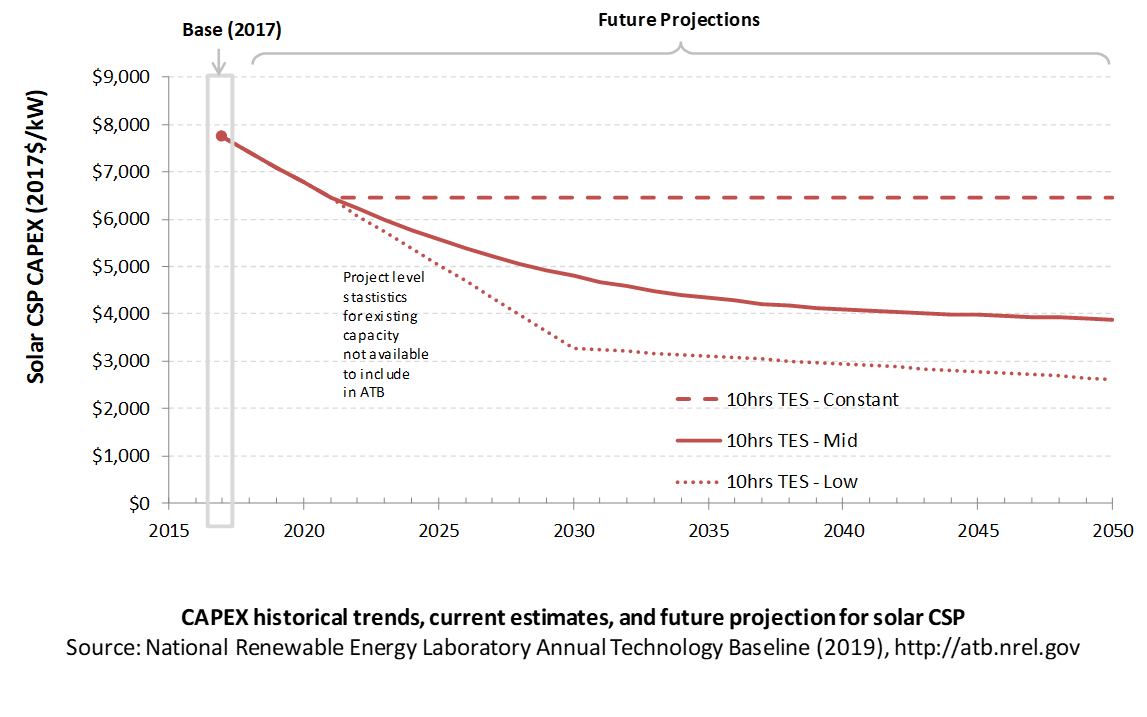
Capital expenditures (CAPEX) are expenditures required to achieve commercial operation in a given year. These expenditures include the generation plant, the balance of system (e.g., site preparation, installation, and electrical infrastructure), and financial costs (e.g., development costs, and interest during construction) and are detailed in CAPEX Definition. In the ATB, CAPEX reflects typical plants and does not include differences in regional costs associated with labor, materials, taxes, or system requirements. The related Standard Scenarios product uses Regional CAPEX Adjustments. The range of CAPEX demonstrates variation with resource in the contiguous United States.
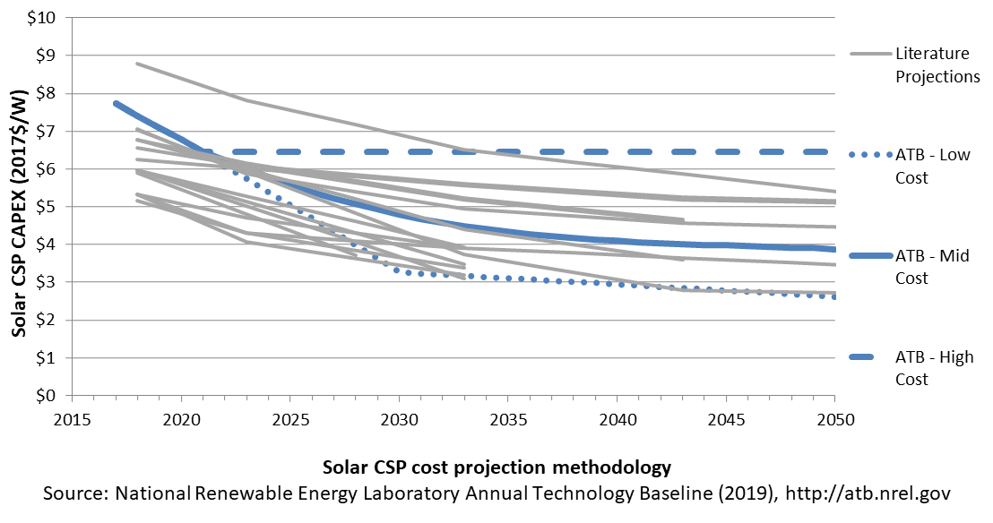
The following figure shows the Base Year estimate and future year projections for CAPEX costs. Three cost scenarios are represented: Constant, Mid, and Low. The estimate for a given year represents CAPEX of a new plant that reaches commercial operation in that year (i.e., SAM 2018 CSP costs are reflected in the ATB in 2021).
Base Year Estimates
CAPEX is unchanged for resource class because the same plant is assumed to be built in each location. The capacity factor will change with resource.
TES increases plant CAPEX but also increases capacity factor and annual efficiency. TES generally lowers LCOE for power towers.
The CAPEX estimate (with a base year of 2017) is approximately $7,730/kWe in 2017$. It is for a representative power tower with 10 hours of storage and a solar multiple of 2.4. Based on recent assessment of the industry in 2017 and updated CSP systems costs reflected in SAM 2018.11.11 (Craig Turchi et al. 2019), the CAPEX estimate for 2021 is $6,450/kWe in 2017$.
Future Year Projections
Three cost projections are developed for CSP technologies:
- Constant Technology Cost Scenario: no change in CAPEX, O&M, or capacity factor from current estimates (2021 for CSP) to 2050; consistent across all renewable energy technologies in the ATB
- The Mid Technology Cost Scenario is based on recently published literature projections and NREL judgment of U.S. costs for future CAPEX at 2025, 2030, 2040 and 2050 ((IRENA 2016), (Breyer et al. 2017), (Murphy et al. 2019), (Feldman et al. 2016), and (World Bank 2014)). It is anticipated that CSP costs could fall by approximately 25% from the ATB CSP 2021 costs of $6,450/kWe to approximately $4,800/kWe by 2030. From 2030 to 2050, CSP CAPEX is projected to fall to approximately $3,380/kWe.
- The Low Technology Cost Scenariois based on the lower bound of the literature sample, and on the Power to Change report (IRENA 2016).
Relative to today's reported CAPEX for plants either announced or in construction, $6,450/kWe in the ATB in 2021 and $4,800/kWe in 2030 is possible. For example, Noor III (150 MWe molten salt power tower with 7.5 hours of storage and operational in 2018), had an estimated CAPEX of $6,500/kWe in 2017$ (Kistner 2016). The Dubai Electricity and Water Authority (DEWA) 700-MWe CSP portion (600-MWe parabolic trough and 100-MWe molten salt tower, each with 12-15 hours of storage), which is in construction had an estimated bundled CAPEX of $5,500/kWe ( (Shemer 2018), (Craig Turchi et al. 2019)).
A detailed description of the methodology for developing future year projections is found in Projections Methodology.
Technology innovations that could impact future O&M costs are summarized in LCOE Projections.
CAPEX Definition
Capital expenditures (CAPEX) are expenditures required to achieve commercial operation in a given year.
The ATB represents the year in which a plant starts commercial operation. Accordingly, for plants whose construction duration exceeds one year, CAPEX costs will represent technology costs that are lagging current-year estimates by at least one year. For CSP plants, the construction period is typically three years.
For the ATB – and based on key sources ((EIA 2016), (C. Turchi 2010), and (Craig Turchi and Heath 2013)) – the CSP generation plant envelope is defined to include:
- CSP generation plant
- Solar collectors
- Solar receiver
- Piping and heat-transfer fluid system
- Power block (heat exchangers, power turbine, generator, and cooling system)
- Thermal energy storage system
- Installation
- Balance of system, including installation, land acquisition, electrical infrastructure, and project indirect costs
- Land acquisition, site preparation, and installation of underground utilities, access roads, fencing, and buildings for operations and maintenance
- Electrical infrastructure, such as transformers, switchgear, and electrical system connecting modules to each other and to control the center; the generator voltage is 13.8 kV, the step-up transformer is 13.8/230kV, and the transmission tie line is 230 kV
- Project indirect costs, including costs related to engineering, distributable labor and materials, construction management start up and commissioning, and contractor overhead costs, fees, and profit
- Financial costs
- Owners' costs, such as development costs, preliminary feasibility and engineering studies, environmental studies and permitting, legal fees, insurance costs, and property taxes during construction
- Onsite electrical equipment (e.g., switchyard), a nominal-distance spur line (< 1 mile), and necessary upgrades at a transmission substation; distance-based spur line cost (GCC) not included in the ATB
- Interest during construction estimated based on three-year duration accumulated 80%/10%/10% at half-year intervals and a nominal interest rate (ConFinFactor).
CAPEX can be determined for a plant in a specific geographic location as follows:
Regional cost variations and geographically specific grid connection costs are not included in the ATB (CapRegMult = 1; GCC = 0). In the ATB, the input value is overnight capital cost (OCC) and details to calculate interest during construction (ConFinFactor).
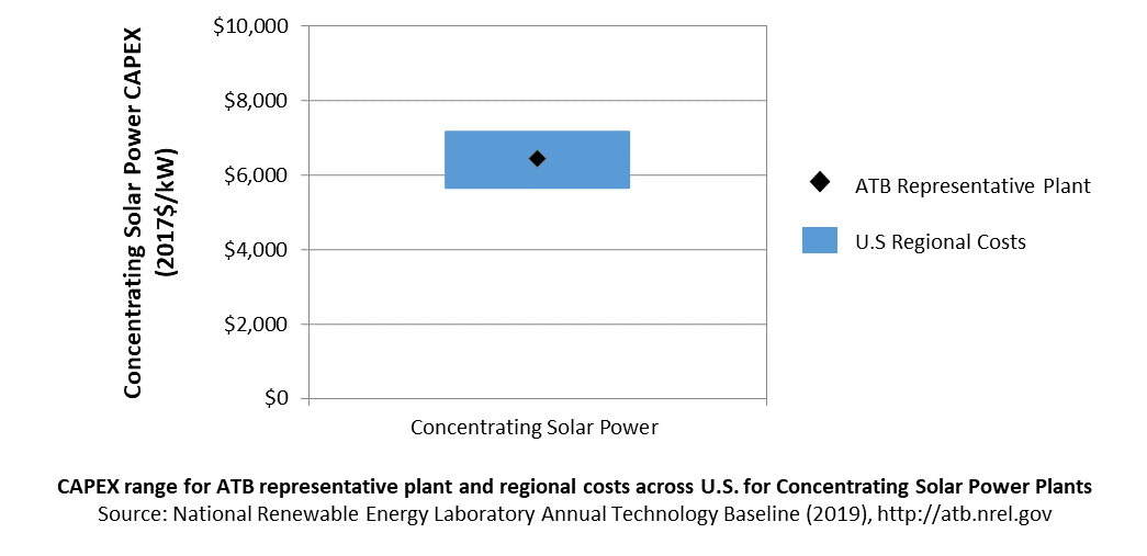
In the ATB, CAPEX represents a typical solar-CSP plant with 10 hours of thermal storage and does not vary with resource. Regional cost effects associated with labor rates, material costs, and other regional effects as defined by the U.S. Energy Information Administration (EIA 2016) expand the range of CAPEX. Unique land-based spur line costs based on distance and transmission line costs expand the range of CAPEX even further. The following figure illustrates the ATB representative plant relative to the range of CAPEX including regional costs across the contiguous United States. The ATB representative plants are associated with a regional multiplier of 1.0.
Standard Scenarios Model Results
ATB CAPEX, O&M, and capacity factor assumptions for the Base Year and future projections through 2050 for Constant, Mid, and Low technology cost scenarios are used to develop the NREL Standard Scenarios using the ReEDS model. See ATB and Standard Scenarios.
CAPEX in the ATB does not represent regional variants (CapRegMult) associated with labor rates, material costs, etc., but the ReEDS model does include 134 regional multipliers (EIA 2016).
The ReEDS model determines the land-based spur line (GCC) uniquely for each potential CSP plant based on distance and transmission line cost.
Operation and Maintenance (O&M) Costs
Operations and maintenance (O&M) costs represent the annual expenditures required to operate and maintain a solar CSP plant over its lifetime, including:
- Operating and administrative labor, insurance, legal and administrative fees, and other fixed costs
- Utilities (water, power, and natural gas if any) and mirror washing
- Scheduled and unscheduled maintenance, including replacement parts for solar field and power block components over the technical lifetime of the plant.
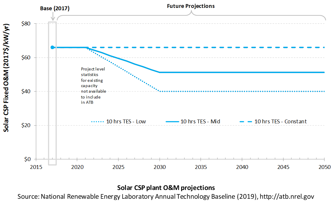
The following figure shows the Base Year estimate and future year projections for fixed O&M (FOM) costs. Three cost scenarios are represented. The estimate for a given year represents annual average FOM costs expected over the technical lifetime of a new plant that reaches commercial operation in that year.
Base Year Estimates
FOM is assumed to be $66/kW-yr until 2021. Variable O&M is approximately $4.1/MWh until 2021 and $3.50/MWh after that (Kurup and Turchi 2015).
Future Year Projections
Future FOM is assumed to decline to $51/kW-yr by 2030 in the Mid cost case (i.e., approximately a 25% drop) and approximately $40/kW-yr by 2030 in the Low cost case based on DOE investments likely to help to lower costs (DOE 2012).
A detailed description of the methodology for developing future year projections is found in Projections Methodology.
Technology innovations that could impact future O&M costs are summarized in LCOE Projections.
Capacity Factor: Expected Annual Average Energy Production Over Lifetime
The capacity factor represents the expected annual average energy production divided by the annual energy production, assuming the plant operates at rated capacity for every hour of the year. It is intended to represent a long-term average over the lifetime of the plant. It does not represent interannual variation in energy production. Future year estimates represent the estimated annual average capacity factor over the technical lifetime of a new plant installed in a given year.
Capacity factors are influenced by power block technology, storage technology and capacity, the solar resource, expected downtime, and energy losses. The solar multiple is a design choice that influences the capacity factor.
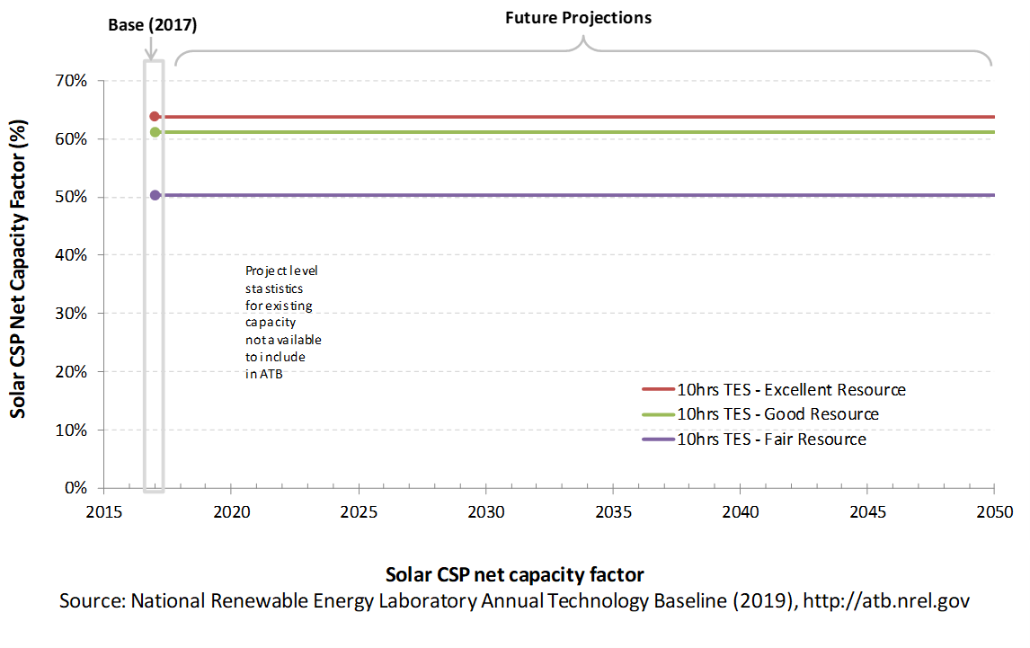
The following figure shows a range of capacity factors based on variation in the resource, for locations where currently CSP plants could be built in the contiguous United States. The range of the Base Year estimates illustrates the effect of locating a CSP plant at a site with Fair, Good, or Excellent solar resource. The future projections for the Constant, Mid, and Low technology cost scenarios are unchanged from the Base Year. Technology improvements are focused on CAPEX and O&M cost elements.
Base Year Estimates
For illustration in the ATB, a range of capacity factors calculated in SAM 2018.11.11 (NREL n.d.) is associated with three resource locations in the contiguous United States, as represented in the ReEDS model for three classes of insolation:
- Fair resource: Abilene, Texas: 6.16 kWh/m2/day based on the site TMY3 file, leads to a 50% capacity factor; the 2017 PSM TMY file for a site adjacent to the airport is used, and it was downloaded from the NSRDB (NREL n.d.).
- Good resource: Phoenix, Arizona: 7.26 kWh/m2/day based on the site TMY3 leads to a 61% capacity factor; the TMY file used is available in SAM 2018.11.11(NREL n.d.), titled "phoenix_az_33.450495_-111.983688_psmv3_60_tmy"..
- Excellent resource: Daggett, California: 7.65 kWh/m2/day based on the site TMY3 file, leads to a 64% capacity factor; the TMY file used is available in SAM 2018.11.11 (NREL n.d.), titled "daggett_ca_34.865371_-116.783023_psmv3_60_tmy".
A key finding from a recent report is that if future costs of CSP decrease sufficiently, it could be deployed across a greater range of the United States and DNI resources. For example, with aggressive cost decreases and due to the regional market constraints, southeastern states with lower DNI resources (e.g., Florida and South Carolina) could see increased CSP capacity deployments of up to 5 GWe (Murphy et al. 2019).
Future Year Projections
The CSP technologies highlighted in the ATB are assumed to be power towers but with different power cycles and operating conditions as time passes:
- 2017: a molten-salt (sodium nitrate/potassium nitrate; aka, solar salt) power tower with direct two-tank TES combined with a steam-Rankine power cycle running at 574° C and 41.2% gross efficiency
- 2021: a similar design to that of 2017 with identified near-term reductions in heliostat and power system costs
- 2030 Mid Technology Cost Scenario: longer-term cost reductions (e.g., in the heliostats and power system)
- 2030 Low Technology Cost Scenario: In the ATB, the Low projection is based on molten-salt power tower with direct two-tank TES combined with a power cycle running at 700° C and 55% gross efficiency.
While an advanced molten salt projection is used for the ATB Low Cost scenario, lower costs for baseload CSP are being investigated via different technology options (i.e. Solid Particle and Gas phase towers) and as defined by the CSP Gen3 program ((EERE n.d.), (Mehos et al. 2017)).
Over time, CSP plant output may decline. Capacity factor degradation due to mirror and other component degradation is not accounted for in ATB estimates of capacity factor or LCOE.
The ATB capacity factors are generated from Constant, Mid and Low technology cost plant simulations in SAM 2018.11.11 (NREL n.d.).
Estimates of capacity factors for CSP in the ATB represent typical operation. The dispatch characteristics of these systems are valuable to the electric system to manage changes in net electricity demand. Actual capacity factors will be influenced by the degree to which system operators call on CSP plants to manage grid services.
Standard Scenarios Model Results
ATB CAPEX, O&M, and capacity factor assumptions for the Base Year and future projections through 2050 for Constant, Mid, and Low technology cost scenarios are used to develop the NREL Standard Scenarios using the ReEDS model. See ATB and Standard Scenarios.
CSP plants with TES can be dispatched by grid operators to accommodate diurnal and seasonal load variations and output from variable generation sources (wind and solar PV). Because of this, their annual energy production and the value of that generation are determined by the electric system needs and capacity and ancillary services markets.
Plant Cost and Performance Projections Methodology
A range of literature projections is shown to illustrate the comparison with the ATB. When comparing the ATB projections with other projections, note that there are major differences in technology assumptions, radiation conditions, field sizes, storage configurations, and other factors. As shown in the chart, the ATB 2019 CSP Mid projection is in line with other recently analyzed projections from other organizations. The Low cost ATB projection is based on the lower bound of the literature sample, and on the Power to Change report (IRENA 2016).
Projections of future utility-scale CSP plant CAPEX and O&M are based on three different technology cost scenarios that were developed for scenario modeling as bounding levels:
- Constant Technology Cost Scenario
- Modeled as molten-salt (sodium nitrate/potassium nitrate, aka, solar salt) power tower with direct two-tank TES combined with a steam-Rankine power cycle running at 574°C and 41.2% gross efficiency in 2017
- Costs stay the same from the 2021 estimate through 2050, consistent with ATB renewable energy technologies
- Mid Technology Cost Scenario:
- Based on recently published literature projections and NREL judgment of U.S. costs for future CAPEX in 2025, 2030, 2040 and 2050 ((IRENA 2016), (Breyer et al. 2017), (Murphy et al. 2019), (Feldman et al. 2016), and (World Bank 2014)).
- It is anticipated that CSP costs could fall by approximately 25% from the ATB CSP 2021 costs of $6,450/kWe to approximately $4,800/kWe by 2030.
- CSP CAPEX is projected to fall from 2030 to 2050 to approximately $3,380/kWe.
- The cost reductions are anticipated due to gradual reductions in heliostat and power system cost due to greater deployment volume and learning assumed for 2021 and onwards based on current state of industry ((IRENA 2016), (Lilliestam et al. 2017)).
- CAPEX and O&M both drop by approximately 25% by 2030, relative to 2021 costs
- A further 30% overall CAPEX decrease is estimated from 2030 to 2050. All three components of the CSP CAPEX (the turbine, storage, and the solar field), decrease proportionately by approximately 30% from 2030 to 2050.
- Low Technology Cost Scenario:
- Significant reductions in heliostat and power system cost due to greater deployment volume and R&D are used for 2021 onwards; the plant was modeled as an advanced molten-salt power tower with direct two-tank TES combined with a power cycle running at 700°C and 55% gross efficiency in 2030 (Mehos et al. 2017).
- CAPEX and O&M decrease from likely cost reductions including new high-efficiency power cycles and low-cost heliostats.
- A further 20% overall CAPEX decrease is assumed from 2030 to 2050 based on potential deployment in the United States. The 20% decrease in overall CSP CAPEX is split over the three components: the turbine, storage, and the solar field. It can be expected that greater cost reductions could be achieved for the power block/turbine and the solar field than for the storage.
Levelized Cost of Energy (LCOE) Projections
Levelized cost of energy (LCOE) is a summary metric that combines the primary technology cost and performance parameters: CAPEX, O&M, and capacity factor. It is included in the ATB for illustrative purposes. The ATB focuses on defining the primary cost and performance parameters for use in electric sector modeling or other analysis where more sophisticated comparisons among technologies are made. The LCOE accounts for the energy component of electric system planning and operation. The LCOE uses an annual average capacity factor when spreading costs over the anticipated energy generation. This annual capacity factor ignores specific operating behavior such as ramping, start-up, and shutdown that could be relevant for more detailed evaluations of generator cost and value. Electricity generation technologies have different capabilities to provide such services. For example, wind and PV are primarily energy service providers, while the other electricity generation technologies such as CSP can provide capacity and flexibility services in addition to energy. These capacity and flexibility services are difficult to value and depend strongly on the system in which a new generation plant is introduced. These services are represented in electric sector models such as the ReEDS model and corresponding analysis results such as the Standard Scenarios.
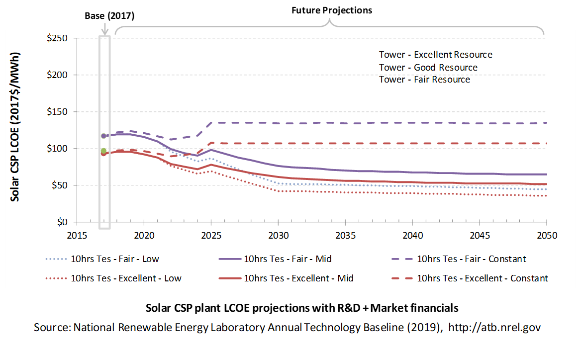
The following three figures illustrate LCOE, which includes the combined impact of CAPEX, O&M, and capacity factor projections for power-tower CSP across the range of resources present in the contiguous United States. For the purposes of the ATB, the costs associated with technology and project risk in the U.S. market are represented in the financing costs but not in the upfront capital costs (e.g., developer fees and contingencies). An individual technology may receive more favorable financing terms outside the United States, due to less technology and project risk, caused by more project development experience (e.g., offshore wind in Europe) or more government or market guarantees. The R&D Only LCOE sensitivity cases present the range of LCOE based on financial conditions that are held constant over time unless R&D affects them, and they reflect different levels of technology risk. This case excludes effects of tax reform, tax credits, and changing interest rates over time. The R&D + Market LCOE case adds to these financial assumptions: (1) the changes over time consistent with projections in the Annual Energy Outlook and (2) the effects of tax reform and tax credits. For example, the projected LCOE for most utility scale renewable energy generation technologies could potentially increase from the end of 2020 due to the decreasing levels of the ITC. The ATB representative plant characteristics that best align with those of recently installed or anticipated near-term CSP plants are associated with Tower-Excellent Resource. Data for all the resource categories can be found in the ATB Data spreadsheet; for simplicity, not all resource categories are shown in the figures.
Note: the future projection of the "Good resource" (i.e., for a CSP plant built in Phoenix, Arizona) is not shown in the figures to simplify the figures and because the projection lies between the Excellent and the Fair Resource projections.
R&D Only | R&D + Market

 R&D + Market
The methodology for representing the CAPEX, O&M, and capacity factor assumptions behind each pathway is discussed in Projections Methodology. In general, the degree of adoption of technology innovation distinguishes the Constant, Mid, and Low technology cost scenarios. These projections represent trends that reduce CAPEX and improve performance. Development of these scenarios involves technology-specific application of the following general definitions:
- Constant Technology: Base Year (or near-term estimates of projects under construction) equivalent through 2050 maintains current relative technology cost differences
- Mid Technology Cost Scenario: Technology advances through continued industry growth, public and private R&D investments, and market conditions relative to current levels that may be characterized as "likely" or "not surprising"
- Low Technology Cost Scenario: Technology advances that may occur with breakthroughs, increased public and private R&D investments, and/or other market conditions that lead to cost and performance levels that may be characterized as the " limit of surprise" but not necessarily the absolute low bound.
To estimate LCOE, assumptions about the cost of capital to finance electricity generation projects are required, and the LCOE calculations are sensitive to these financial assumptions. Two project finance structures are used within the ATB:
- R&D Only Financial Assumptions: This sensitivity case allows technology-specific changes to debt interest rates, return on equity rates, and debt fraction to reflect effects of R&D on technological risk perception, but it holds background rates constant at 2017 values from AEO2019 (EIA 2019) and excludes effects of tax reform and tax credits.
- R&D Only + Market Financial Assumptions: This sensitivity case retains the technology-specific changes to debt interest, return on equity rates, and debt fraction from the R&D Only case and adds in the variation over time consistent with AEO2019 (EIA 2019) as well as effects of tax reform and tax credits. For a detailed discussion of these assumptions, see Project Finance Impact on LCOE.
A constant cost recovery period – over which the initial capital investment is recovered – of 30 years is assumed for all technologies throughout this website, and can be varied in the ATB data spreadsheet.
The equations and variables used to estimate LCOE are defined on the Equations and Variables page. For illustration of the impact of changing financial structures such as WACC, see Project Finance Impact on LCOE. For LCOE estimates for the Constant, Mid, and Low technology cost scenarios for all technologies, see 2019 ATB Cost and Performance Summary.
For illustration of the impact of changing financial structures such as WACC, see Project Finance Impact on LCOE. For LCOE estimates for the Constant, Mid, and Low technology cost scenarios for all technologies, see 2019 ATB Cost and Performance Summary.
In general, differences among the technology cost cases reflect different levels of adoption of innovations. Reductions in technology costs reflect the cost reduction opportunities that are listed below.
- Power tower improvements
- Better and longer-lasting selective surface coatings improve receiver efficiency and reduce O&M costs.
- New salts allow for higher operating temperatures and lower-cost TES.
- Development of the power cycle running at approximately 700°C and 55% gross efficiency improves cycle efficiency, reduces powerblock cost, and reduces O&M costs.
- Lower-cost heliostats developed due to design changes and automated and high-volume manufacturing.
- General and "soft" costs improvements
- Expansion of world market leads to greater and more efficient supply chains, and reduction of supply chain margins (e.g., profit and overhead charged by suppliers, manufacturer, distributors, and retailers).
- Expansion of access to a range of innovative financing approaches and business models
- The LCOE range shown is based on locations with Fair (Abilene, Texas), Good (Phoenix, Arizona), and Excellent (Daggett, California) resources. The CAPEX is the same for each resource as the same plant is used. Future-year LCOE projections for the Good case are not shown to simplify the figure. Using the R&D Only scenario and financials, and with the capacity factor of 64% for Daggett, California (NREL n.d.), in the Mid case by 2030, the LCOE could reach approximately 55$/MWh, and it could potentially reach $47/MWh by 2050.
Hydropower
Renewable energy technical potential, as defined by Lopez et al. (2012) , represents the achievable energy generation of a particular technology given system performance, topographic limitations, and environmental and land-use constraints. The primary benefit of assessing technical potential is that it establishes an upper-boundary estimate of development potential. It is important to understand that there are multiple types of potential-resource, technical, economic, and market (see NREL: "Renewable Energy Technical Potential").
Note: Pumped-storage hydropower is considered a storage technology in the ATB and will be addressed in future years. It and other storage technologies are represented in Standard Scenarios Model Results from the ReEDS model, and battery storage technologies are shown in the associated portion of the ATB.
Representative Technology
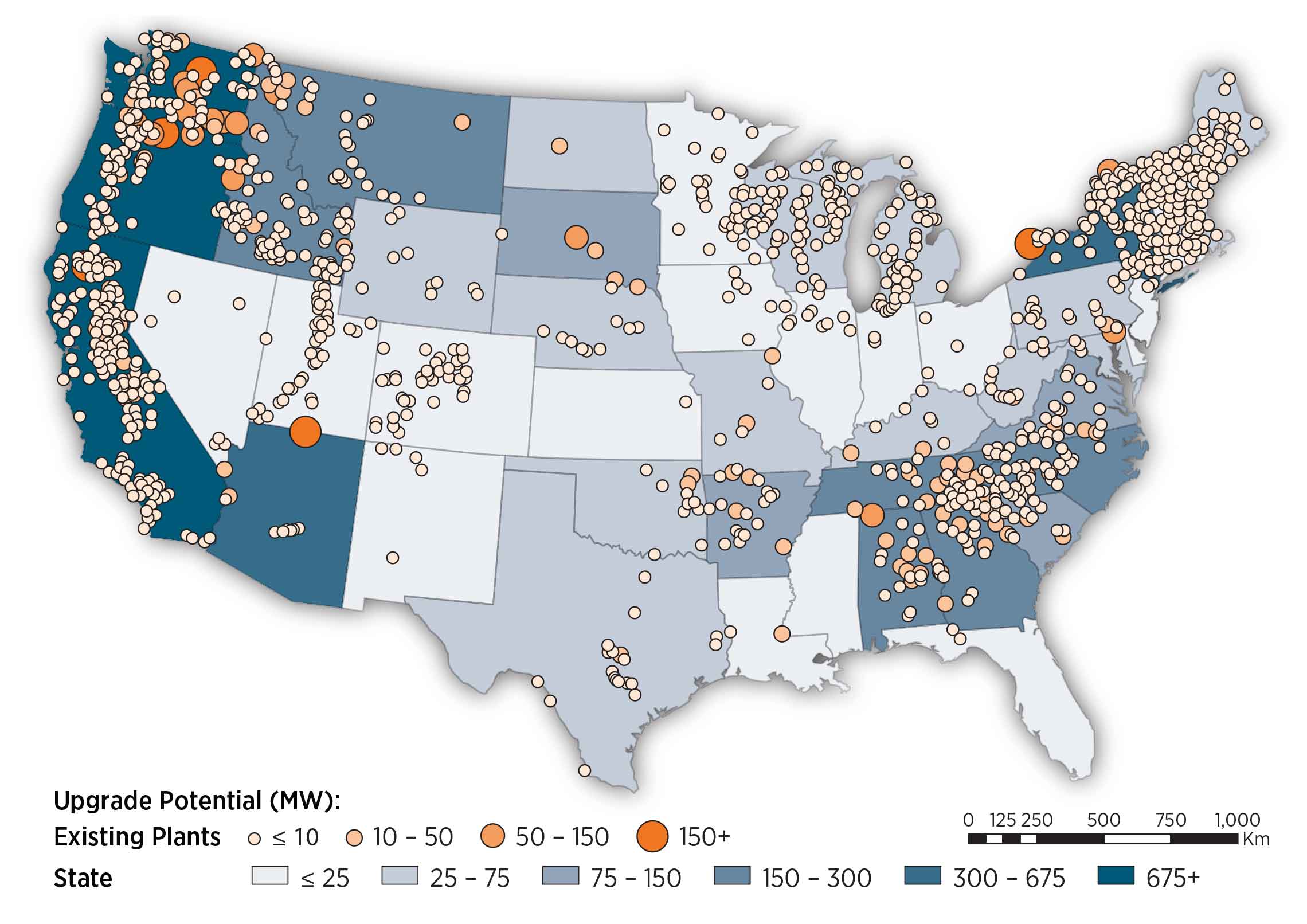
Hydropower technologies have produced electricity in the United States for over a century. Many of these infrastructure investments have potential to continue providing electricity in the future through upgrades of existing facilities (DOE, 2016) . At individual facilities, investments can be made to improve the efficiency of existing generating units through overhauls, generator rewinds, or turbine replacements. Such investments are known collectively as "upgrades," and they are reflected as increases to plant capacity. As plants reach a license renewal period, upgrades to existing facilities to increase capacity or energy output are typically considered. While the smallest projects in the United States can be as small as 10-100 kW, the bulk of upgrade potential is from large, multi-megawatt facilities.
Resource Potential
The estimated total upgrade potential of 6.9 GW/24 terawattt-hours (TWh) (at about 1,800 facilities) is based on generalizable information drawn from a series of case studies or owner-specific assessments (DOE, 2016) . Information available to inform the representation of improvements to the existing fleet includes:
- A systematic, full-fleet assessment of expansion potential at Reclamation projects performed under the Reclamation Hydropower Modernization Initiative (see U.S. Bureau of Reclamation, "Hydropower Resource Assessment at Existing Reclamation Facilities")
- Case study reports from the U.S. Army Corps of Engineers (Corps) performed under its Hydropower Modernization Initiative (MWH, Watson, & Harza, 2009)
- Case study reports combining assessments of upgrade and unit and plant optimization potential from the U.S. Department of Energy/Oak Ridge National Laboratory Hydropower Advancement Project.
Base Year and Future Year Projections Overview
Upgrades are often among the lowest-cost new capacity resource, with the modeled costs for individual projects ranging from $800/kW to nearly $20,000/kW. This differential results from significant economies of scale from project size, wherein larger capacity plants are less expensive to upgrade on a dollar-per-kilowatt basis than smaller projects are. The average cost of the upgrade resource is approximately $1,500/kW.
CAPEX for each existing facility is based on direct estimates
The capacity factor is based on actual 10-year average energy production reported in EIA 923 forms. Some hydropower facilities lack flexibility and only produce electricity when river flows are adequate. Others with storage capabilities are operated to meet a balance between electric system, reservoir management, and environmental needs using their dispatch capability.
No future cost and performance projections for hydropower upgrades are assumed.
Upgrade cost and performance are not illustrated in this documentation of the ATB for the sake of simplicity.
Standard Scenarios Model Results
ATB CAPEX, O&M, and capacity factor assumptions for the Base Year and future projections through 2050 for Constant, Mid, and Low technology cost scenarios are used to develop the NREL Standard Scenarios using the ReEDS model. See ATB and Standard Scenarios.
Upgrade potential becomes available in the ReEDS model at the relicensing date, end of plant life (50 years), or both.

Representative Technology
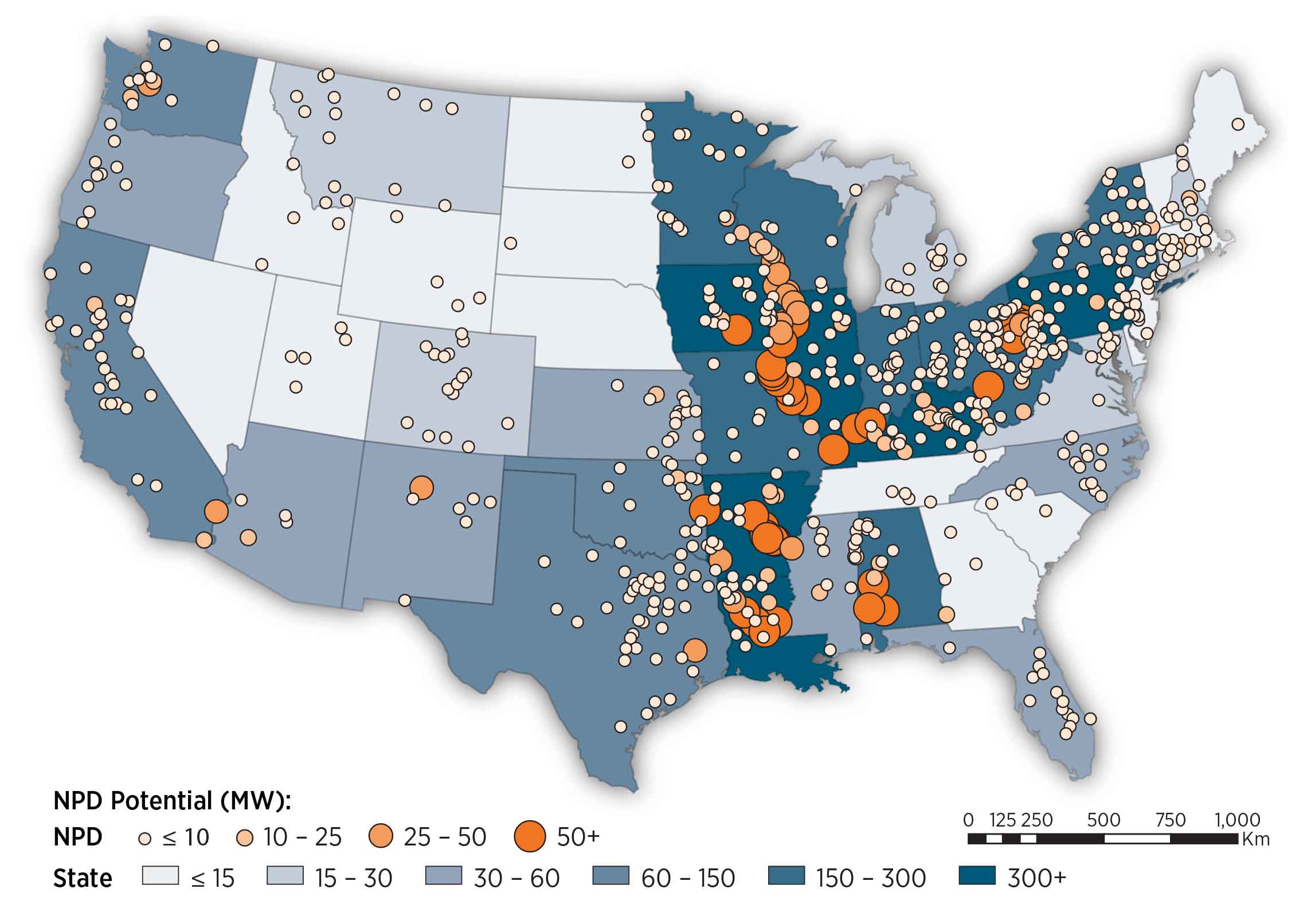
Non-powered dams (NPD) are classified by energy potential in terms of head. Low head facilities have design heads below 20 m and typically exhibit the following characteristics (DOE, 2016) :
- 1 MW to 10 MW
- New/rehabilitated intake structure
- Little, if any, new penstock
- Axial-flow or Kaplan turbines (2-4 units)
- New powerhouse (indoor)
- New/rehabilitated tailrace
- Minimal new transmission (< 5 miles, if required)
- Capacity factor of 35% to 60%.
High head facilities have design heads above 20 m and typically exhibit the following characteristics (DOE, 2016) :
- 5 MW to 30 MW
- New/rehabilitated intake structure
- New penstock (typically < 500 feet of steel penstock, if required)
- Francis turbines (1-3 units)
- New powerhouse (indoor)
- New/rehabilitated tailrace
- Minimal new transmission line (up to 15 MW, if required)
- Capacity factor of 35% to 60%.
Resource Potential
Up to 12 GW of technical potential exists to add power to U.S. NPD. However, based on financial decisions in recent development activity, the economic potential of NPD may be approximately 5.6 GW at more than 54,000 dams in the contiguous United States. Most of this potential (5 GW or 90% of resource capacity) is associated with less than 700 dams. These resource considerations are discussed below:
According to the National
Inventory of Dams, more than 80,000 dams exist that do not produce
power. This data set was filtered to remove dams with erroneous flow
and geographic data and dams whose data could not be resolved to a
satisfactory level of detail
A new methodology for sizing potential hydropower facilities that was developed for the new-stream reach development resource (Kao et al., 2014) was applied to non-powered dams. This resource potential was estimated to be 5.6 GW at more than 54,000 dams. In the development of the Hydropower Vision, the NPD resource available to the ReEDS model was adjusted based on recent development activity and limited to only those projects with power potential of 500 kW or more. As the ATB uses the Hydropower Vision supply curves, this results in a final resource potential of 5 GW/29 TWh from 671 dams.
For each facility, a design capacity, average monthly flow rate over a 30-year period, and a design flow rate exceedance level of 30% are assumed. The exceedance level represents the fraction of time that the design flow is exceeded. This parameter can be varied and results in different capacity and energy generation for a given site. The value of 30% was chosen based on industry rules of thumb. The capacity factor for a given facility is determined by these design criteria.
Design capacity and flow rate dictate capacity and energy generation potential. All facilities are assumed sized for 30% exceedance of flow rate based on long-term, average monthly flow rates.
Base Year and Future Year Projections Overview
Site-specific CAPEX, O&M, and capacity factor estimates are made
for each site in the available resource potential. CAPEX and O&M
estimates are made based on statistical analysis of historical plant
data from 1980 to 2015
Projections developed for the Hydropower Vision study (DOE, 2016) using technological learning assumptions and bottom-up analysis of process and/or technology improvements provide a range of future cost outcomes. Three different projections were developed for scenario modeling as bounding levels:
- Constant Technology Cost Scenario: no change in CAPEX, O&M, or capacity factor from 2017 to 2050; consistent across all renewable energy technologies in the ATB
- Mid Technology Cost Scenario: incremental technology learning, consistent with Reference in Hydropower Vision (DOE, 2016); CAPEX reductions for new stream-reach development (NSD) only
- Low cost: gains that are achievable when pushing to the limits of potential new technologies, such as modularity (in both civil structures and power train design), advanced manufacturing techniques, and materials, consistent with Advanced Technology in Hydropower Vision (DOE, 2016); both CAPEX and O&M cost reductions implemented.
Standard Scenarios Model Results
ATB CAPEX, O&M, and capacity factor assumptions for the Base Year and future projections through 2050 for Constant, Mid, and Low technology cost scenarios are used to develop the NREL Standard Scenarios using the ReEDS model. See ATB and Standard Scenarios.
The ReEDS model includes a sensitivity scenario that restricts the resource potential to sites greater than 500 kW, consistent with the Hydropower Vision, which results in 5 GW/29 TWh at 671 dams.
Representative Technology
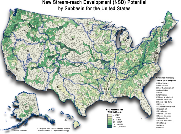
Greenfield or new stream-reach development (NSD) sites are defined as new hydropower developments along previously undeveloped waterways and typically exhibit the following characteristics (DOE, 2016) :
- 1 MW to 100 MW
- New diversion/intake structure
- New penstock
- Steel with length being head/terrain dependent
- Various turbine selections
- Impulse/Francis are common for recently completed projects
- New powerhouse (indoor)
- New tailrace
- New transmission line (up to 15 miles for new projects)
- 30% to 80% capacity factor.
Resource Potential
The resource potential is estimated to be 53.2 GW/301 TWh at nearly 230,000 individual sites (Kao et al., 2014) after accounting for locations statutorily excluded from hydropower development such as national parks, wild and scenic rivers, and wilderness areas.
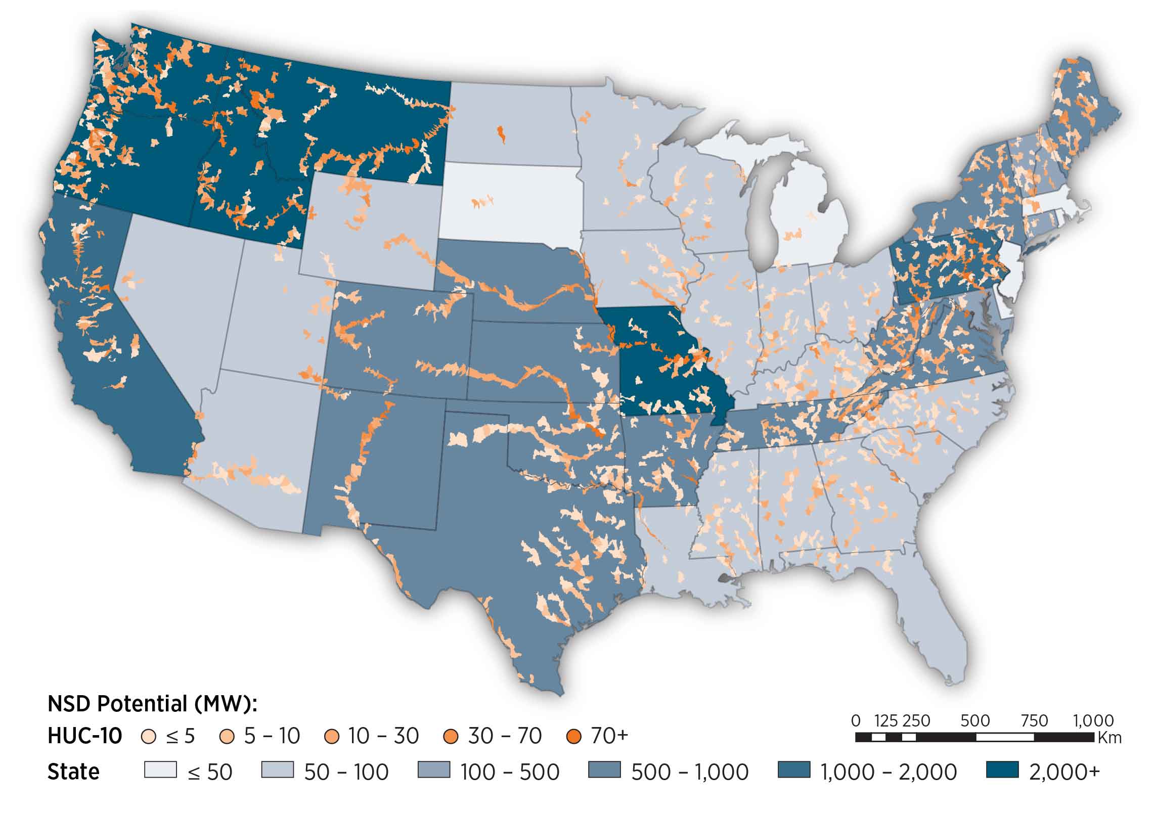
About 8,500 stream reaches were evaluated to assess resource potential (i.e., capacity) and energy generation potential (i.e., capacity factor). For each stream reach, a design capacity, average monthly flow rate over a 30-year period, and design flow rate exceedance level of 30% are assumed. The exceedance level represents the fraction of time that the design flow is exceeded. This parameter can be varied and results in different capacity and energy generation for a given site. The value of 30% was chosen based on industry rules of thumb. The capacity factor for a given facility is determined by these design criteria. Plant sizes range from kilowatt-scale to multi-megawatt scale (Kao et al., 2014) .
The resource assessment approach is designed to minimize the footprint of a hydropower facility by restricting inundation area to the Federal Emergency Management Agency (FEMA) 100-year floodplain.
New hydropower facilities are assumed to apply run-of-river operation strategies. Run-of-river operation means the flow rate into a reservoir is equal to the flow rate out of the facility. These facilities do not have dispatch capability.
Design capacity and flow rate dictate capacity and energy generation potential. All facilities are assumed sized for 30% exceedance of flow rate based on long-term, average monthly flow rates.
Base Year and Future Year Projections Overview
Site-specific CAPEX, O&M, and capacity factor estimates are made
for each site in the available resource potential. CAPEX and O&M
estimates are made based on statistical analysis of historical plant
data from 1980 to 2015
Projections developed for the Hydropower Vision study (DOE, 2016) using technological learning assumptions and bottom-up analysis of process and/or technology improvements provide a range of future cost outcomes. Three different projections were developed for scenario modeling as bounding levels:
- Constant Technology Cost Scenario: no change in CAPEX, O&M, or capacity factor from 2017 to 2050; consistent across all renewable energy technologies in the ATB
- Mid Technology Cost Scenario: incremental technology learning, consistent with Reference in Hydropower Vision (DOE, 2016); CAPEX reductions for NSD only
- Low Technology Cost Scenario: gains that are achievable
when pushing to the limits of potential new technologies, such as
modularity (in both civil structures and power train design), advanced
manufacturing techniques, and materials, consistent with Advanced
Technology in Hydropower Vision
(DOE, 2016) ; both CAPEX and O&M cost reductions implemented.
Standard Scenarios Model Results
ATB CAPEX, O&M, and capacity factor assumptions for the Base Year and future projections through 2050 for Constant, Mid, and Low technology cost scenarios are used to develop the NREL Standard Scenarios using the ReEDS model. See ATB and Standard Scenarios.
The ReEDS model includes a sensitivity scenario that restricts the resource potential to sites greater than 1 MW, which results in 30.1 GW/176 TWh on nearly 8,000 reaches.
Capital Expenditures (CAPEX): Historical Trends, Current Estimates, and Future Projections
Capital expenditures (CAPEX) are expenditures required to achieve commercial operation in a given year. These expenditures include the hydropower generation plant, the balance of system (e.g., site preparation, installation, and electrical infrastructure), and financial costs (e.g., development costs, onsite electrical equipment, and interest during construction) and are detailed in CAPEX Definition. In the ATB, CAPEX reflects typical plants and does not include differences in regional costs associated with labor, materials, taxes, or system requirements. The related Standard Scenarios product uses regional CAPEX adjustments. The range of CAPEX demonstrates variation with resource in the contiguous United States.
The following figure shows the Base Year estimate and future year projections for CAPEX costs. Mid and Low technology cost scenarios are shown. Historical data from actual and proposed non-powered dam (NPD) and new stream-reach development (NSD) plants installed in the United States from 1981 to 2014 are shown for comparison to the ATB Base Year. The estimate for a given year represents CAPEX of a new plant that reaches commercial operation in that year.
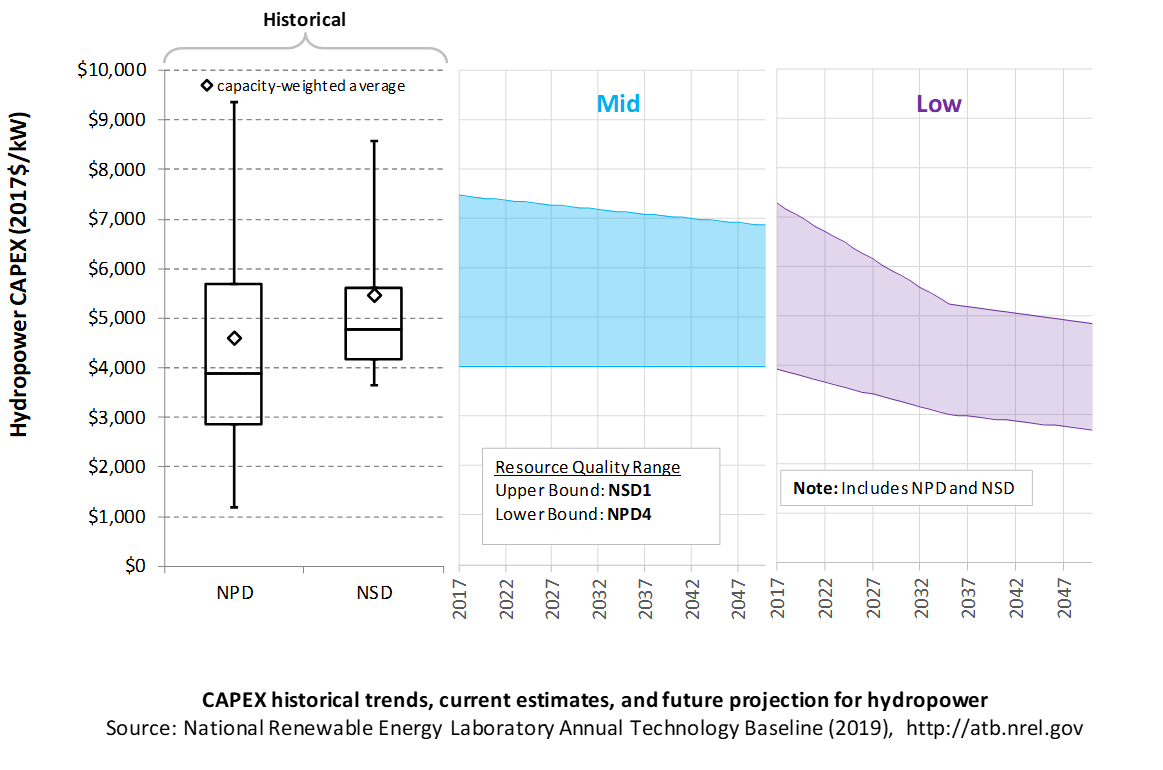
Recent Trends
Actual and proposed NPD and NSD CAPEX from 1981 to 2014
The higher-cost ATB sites generally reflect small-capacity, low head sites that are not comparable to the historical data sample's generally larger-capacity and higher head facilities. These characteristics lead to higher ATB Base Year CAPEX estimates than past data suggest. For example, the NSD projects that became commercially operational in this period are dominated by a few high head projects in the mountains of the Pacific Northwest or Alaska.
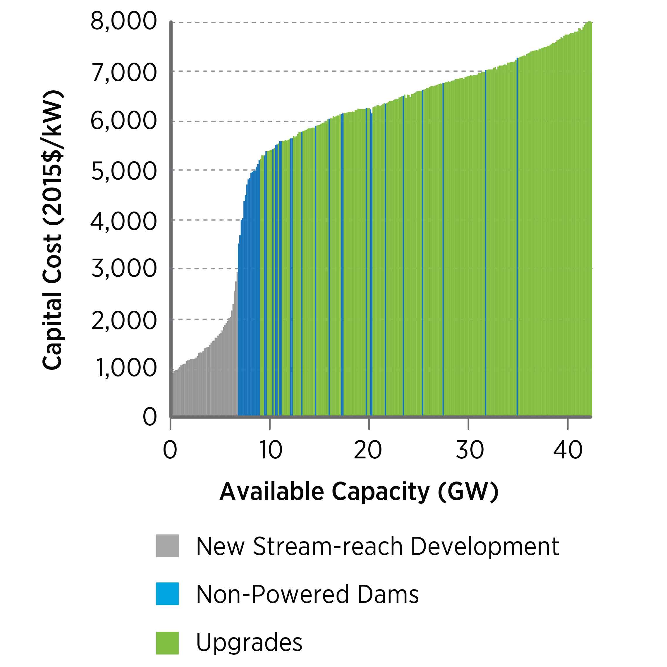
The Base Year estimates of CAPEX for NPDs in the ATB range from $3,800/kW to $6,000/kW. These estimates reflect facilities with 3 feet of head to more than 60 feet of head and from 0.5 MW to more than 30 MW of capacity. In general, the higher-cost sites reflect much smaller-capacity (< 10 MW), lower head (< 30 ft.) sites that have fewer analogues in the historical data, but these characteristics result in higher CAPEX.
The Base Year estimates of CAPEX for NSD range from $5,500/kW to $7,900/kW. The estimates reflect potential sites with 3 feet of head to more than 60 feet head and from 1 MW to more than 30 MW of capacity. In general, NSD potential represents smaller-capacity facilities with lower head than most historical data represent. These characteristics lead to higher CAPEX estimates than past data suggest, as many of the larger, higher head sites in the United States have been previously developed.
Base Year Estimates
For illustration in the ATB, all potential NPD and NSD sites were first binned by both head and capacity. Analysis of these bins provided groupings that represent the most realistic conditions for future hydropower deployment. The design values of these four reference NPD and four reference NSD plants are shown below. The full range of resource and design characteristics is summarized in the ATB data spreadsheet.
Representative Hydropower Plants
| Resource Characteristics Ranges | Weighted Average Values | Calculated Plant Values | |||||
| Plants | Head (feet) | Capacity (MW) | Head (feet) | Capacity (MW) | Capacity Factor | ICC (2014$/kW) | O&M (2014$/kW) |
| NPD 1 | 3-30 | 0.5-10 | 15.4 | 4.8 | 0.62 | 5,969.33 | 111.73 |
| NPD 2 | 3-30 | 10+ | 15.9 | 82.2 | 0.64 | 5,433.24 | 30.74 |
| NPD 3 | 30+ | 0.5-10 | 89.6 | 4.2 | 0.60 | 3,997.79 | 118.67 |
| NPD 4 | 30+ | 10+ | 81.3 | 44.7 | 0.60 | 3,769.22 | 40.54 |
| NSD 1 | 3-30 | 1-10 | 15.7 | 3.7 | 0.66 | 7,034.81 | 125.01 |
| NSD 2 | 3-30 | 10+ | 19.6 | 44.1 | 0.66 | 6,280.15 | 40.76 |
| NSD 3 | 30+ | 1-10 | 46.8 | 4.3 | 0.62 | 6,151.05 | 117.61 |
| NSD 4 | 30+ | 10+ | 45.3 | 94.0 | 0.66 | 5,537.34 | 28.93 |
The reference plants shown above were developed using the average characteristics (weighted by capacity) of the resource plants within each set of ranges. For example, NPD 1 is constructed from the capacity-weighted average values of NPD sites with 3-30 feet of head and 0.5-10 MW of capacity.
The weighted-average values were used as input to the cost formulas
CAPEX for each plant is based on statistical analysis of historical
plant data from 1980 to 2015 as a function of key design parameters,
plant capacity, and hydraulic head
and
Where P is capacity in megawatts, and H is head in feet. The first term represents the initial capital costs, while the second represents licensing.
Future Projections
Projections developed for the Hydropower Vision study (DOE, 2016) using technological learning assumptions and bottom-up analysis of process and/or technology improvements provide a range of future cost outcomes. Three different CAPEX projections were developed for scenario modeling as bounding levels:
- Constant Technology Cost Scenario:
- NPD and NSD CAPEX unchanged from the Base Year; consistent across all renewable energy technologies in the ATB
- Mid Technology Cost Scenario: consistent with the Reference case in Hydropower Vision:
- NSD CAPEX reduced 5% in 2035 and 8.6% in 2050
- NPD CAPEX unchanged from the Base Year
- Low Technology Cost Scenario: consistent with the Advanced Technology case in Hydropower Vision:
- Low head NPD/All NSD CAPEX reduced 30% in 2035 and 35.3% in 2050. Low Head NPD is NPD-1 and NPD-2
- High head NPD CAPEX reduced 25% in 2035 and 32.7% in 2050; High Head NPD is NPD-3 and NPD-4
A detailed description of the methodology for developing future year projections is found in Projections Methodology.
Technology innovations that could impact future O&M costs are summarized in LCOE Projections.
Standard Scenarios Model Results
ATB CAPEX, O&M, and capacity factor assumptions for the Base Year and future projections through 2050 for Constant, Mid, and Low technology cost scenarios are used to develop the NREL Standard Scenarios using the ReEDS model. See ATB and Standard Scenarios.
The ReEDS model uses resource/cost supply curves representing estimates at each individual facility (~700 NPD and ~8,000 NSD).
The ReEDS model represents cost and performance for NPD and NSD potential in 5 bins for each of 134 geographic regions, which results in CAPEX ranges of $2,750/kW-$9,000/kW for NPD resource and $5,200/kW-$15,600/kW for NSD.
CAPEX Definition
Capital expenditures (CAPEX) are expenditures required to achieve commercial operation in a given year.
For the ATB, and based on (EIA, 2016) and the System Cost Breakdown Structure described by (O'Connor, Zhang, DeNeale, Chalise, & Centurion, 2015), the hydropower plant envelope is defined to include:
- Hydropower generation plant
- Civil works, such as site preparation, dams and reservoirs, water conveyances, and powerhouse structures
- Equipment, such as the powertrain and ancillary plant electrical and mechanical systems
- Balance of system (BOS)
- Installation and O&M infrastructure
- Electrical infrastructure, such as transformers, switchgear, and electrical system connecting turbines to each other and to the control center
- Project indirect costs, including costs related to environmental mitigation and regulatory compliance, engineering, distributable labor and materials, construction management start up and commissioning, and contractor overhead costs, fees, and profit
- Financial costs
- Owners' costs, such as development costs, preliminary feasibility and engineering studies, environmental studies and permitting, legal fees, insurance costs, and property taxes during construction
- Electrical interconnection and onsite electrical equipment (e.g., switchyard), a nominal-distance spur line (< 1 mile), and necessary upgrades at a transmission substation; distance-based spur line cost (GCC) not included in the ATB
- Interest during construction estimated based on three-year duration accumulated 10%/10%/80% at half-year intervals and an 8% interest rate (ConFinFactor).
CAPEX can be determined for a plant in a specific geographic location as follows:
Regional cost variations and geographically specific grid connection costs are not included in the ATB (CapRegMult = 1; GCC = 0). In the ATB, the input value is overnight capital cost (OCC) and details to calculate interest during construction (ConFinFactor).
In the ATB, CAPEX is shown for four representative non-powered dam plants and four representative new stream-reach development plants. CAPEX estimates for all identified hydropower potential (~700 NPD and ~8,000 NSD) results in a CAPEX range that is much broader than that shown in the ATB. It is unlikely that all the resource potential will be developed due to the very high costs for some sites. Regional cost effects and distance-based spur line costs are not estimated.
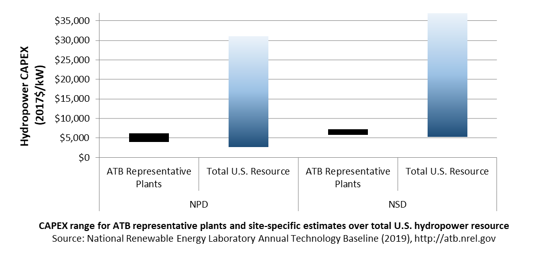
Standard Scenarios Model Results
ATB CAPEX, O&M, and capacity factor assumptions for the Base Year and future projections through 2050 for Constant, Mid, and Low technology cost scenarios are used to develop the NREL Standard Scenarios using the ReEDS model. See ATB and Standard Scenarios.
CAPEX in the ATB does not represent regional variants (CapRegMult) associated with labor rates, material costs, etc., and neither does the ReEDS model.
CAPEX in the ATB does not include geographically determined spur line (GCC) from plant to transmission grid, and neither does the ReEDS model.
Operation and Maintenance (O&M) Costs
Operations and maintenance (O&M) costs represent average annual fixed expenditures (and depend on rated capacity) required to operate and maintain a hydropower plant over its lifetime, including:
- Insurance, taxes, land lease payments, and other fixed costs
- Present value and annualized large component overhaul or replacement costs over technical life (e.g., rewind stator, patch cavitation damage, and replace bearings)
- Scheduled and unscheduled maintenance of hydropower plant components, including turbines, generators, etc. over the technical lifetime of the plant.
The following figure shows the Base Year estimate and future year projections for fixed O&M (FOM) costs. Mid and Low technology cost scenarios are shown. The estimate for a given year represents annual average FOM costs expected over the technical lifetime of a new plant that reaches commercial operation in that year.
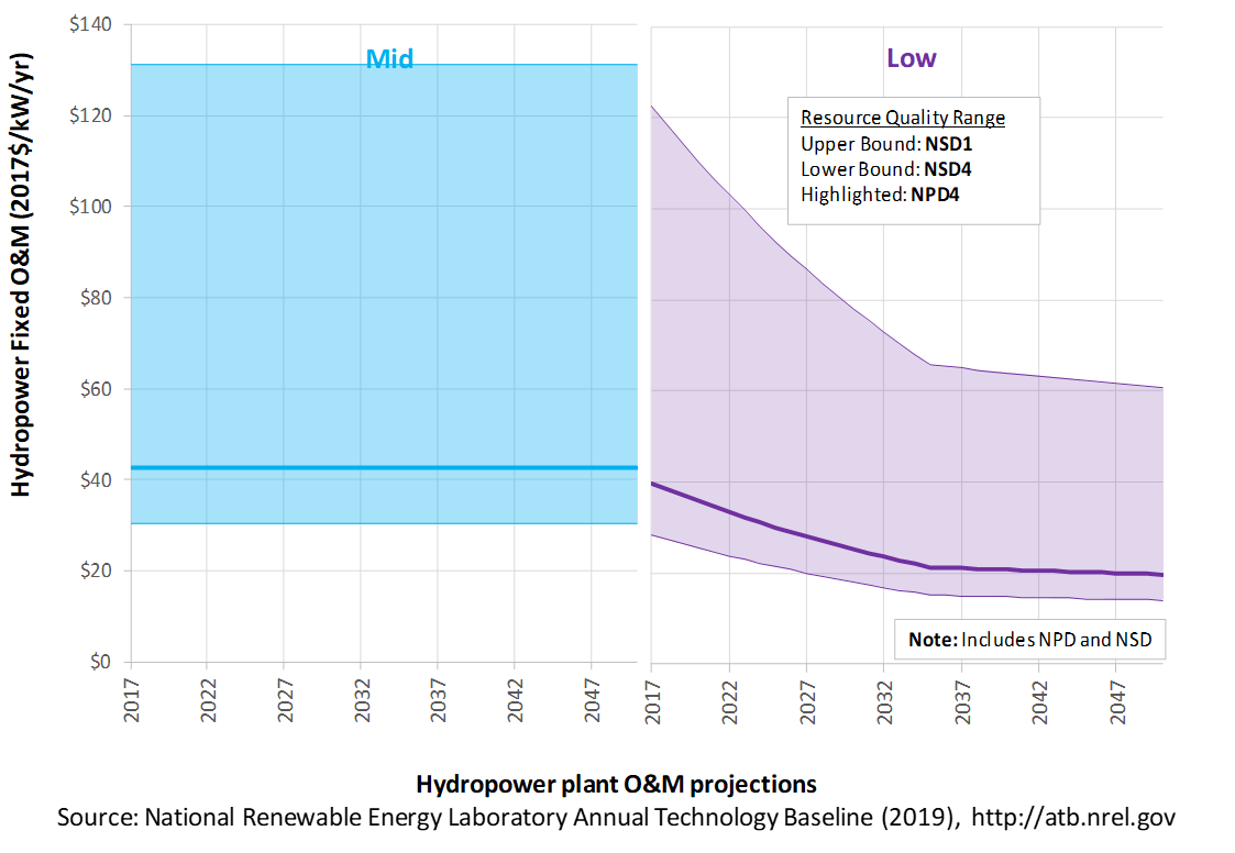
Base Year Estimates
A statistical analysis of long-term plant operation costs from Federal Energy Regulatory Commission Form-1 resulted in a relationship between annual, FOM costs, and plant capacity. Values were updated to 2017$.
Future Year Projections
Projections developed for the Hydropower Vision study (DOE, 2016) using technological learning assumptions and bottom-up analysis of process and/or technology improvements provide a range of future cost outcomes. Three different O&M projections were developed for scenario modeling as bounding levels:
- Constant Technology Cost Scenario: FOM costs unchanged from the Base Year to 2050; consistent with all ATB technologies
- Mid Technology Cost Scenario: FOM costs for both NPD and NSD plants are unchanged from 2017 to 2050; consistent with the Reference case in Hydropower Vision
- Low Technology Cost Scenario: FOM costs for both NPD and NSD plants are reduced by 50% in 2035 and 54% in 2050, consistent with the Advanced Technology case in Hydropower Vision.
A detailed description of the methodology for developing future year projections is found in Projections Methodology.
Technology innovations that could impact future O&M costs are summarized in LCOE Projections.
Capacity Factor: Expected Annual Average Energy Production Over Lifetime
The capacity factor represents the expected annual average energy production divided by the annual energy production, assuming the plant operates at rated capacity for every hour of the year. It is intended to represent a long-term average over the lifetime of the plant. It does not represent interannual variation in energy production. Future year estimates represent the estimated annual average capacity factor over the technical lifetime of a new plant installed in a given year.
The capacity factor is influenced by site hydrology, design factors (e.g., exceedance level), and operation characteristics (e.g., dispatch or run-of-river). Capacity factors for all potential NPD sites and NSDs are estimated based on design criteria, long-term monthly flow rate records, and run-of-river operation.
The following figure shows a range of capacity factors based on variation in the resource for hydropower plants in the contiguous United States. Historical data from run-of-river hydropower plants operating in the United States from 2003 through 2012 are shown for comparison with the Base Year estimates. The range of the Base Year estimates illustrates the effect of resource variation. Future projections for the Constant, Mid, and Low technology cost scenarios are unchanged from the Base Year. Technology improvements are focused on CAPEX and O&M cost elements.
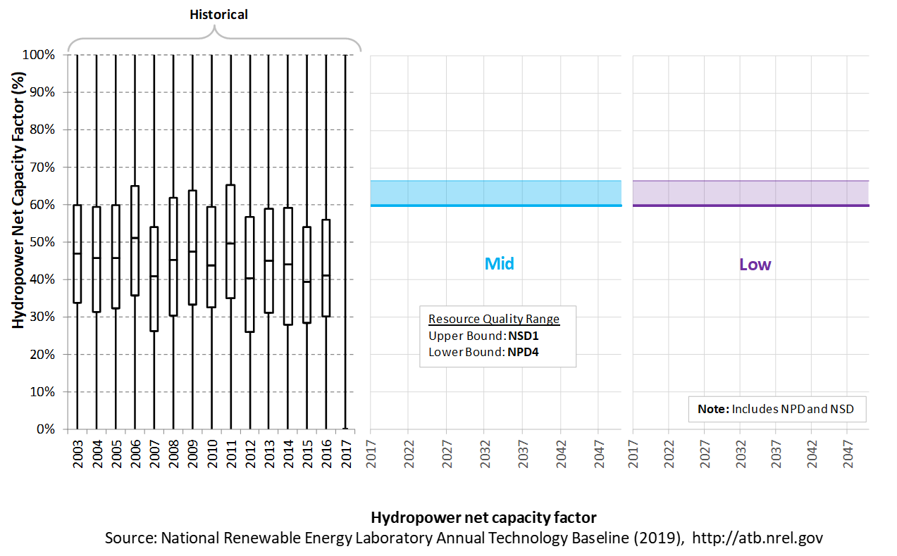
Recent Trends
Actual energy production from about 200 run-of-river plants operating in the United States from 2003 to 2012 (EIA, 2016) is shown in box-and-whiskers format for comparison with current estimates and future projections. This sample includes some very old plants that may have lower availability and efficiency. It also includes plants that have been relicensed and may no longer be optimally designed for current operating regime (e.g., a peaking unit now operating as run-of-river). This contributes to the broad range, particularly on the low end.
Interannual variation of hydropower plant output for run-of-river plants may be significant due to hydrological changes such as drought. This impact may be exacerbated by climate change over the long term.
Current and future estimates for new hydropower plants are within the range of observed plant performance. These potential hydropower plants would be designed for specific site conditions, which would indicate operation toward the high end of the range.
Base Year Estimates
For illustration in the ATB, all potential NPD and NSD sites are represented with four reference plants, each as described below.
Representative Hydropower Plants
| Resource Characteristics Ranges | Weighted Average Values | Calculated Plant Values | |||||
| Plants | Head (feet) | Capacity (MW) | Head (feet) | Capacity (MW) | Capacity Factor | ICC (2014$/kW) | O&M (2014$/kW) |
| NPD 1 | 3-30 | 0.5-10 | 15.4 | 4.8 | 0.62 | 5,969.33 | 111.73 |
| NPD 2 | 3-30 | 10 + | 15.9 | 82.2 | 0.64 | 5,433.24 | 30.74 |
| NPD 3 | 30 + | 0.5-10 | 89.6 | 4.2 | 0.60 | 3,997.79 | 118.67 |
| NPD 4 | 30 + | 10 + | 81.3 | 44.7 | 0.60 | 3,769.22 | 40.54 |
| NSD 1 | 3-30 | 1-10 | 15.7 | 3.7 | 0.66 | 7,034.81 | 125.01 |
| NSD 2 | 3-30 | 10 + | 19.6 | 44.1 | 0.66 | 6,280.15 | 40.76 |
| NSD 3 | 30 + | 1-10 | 46.8 | 4.3 | 0.62 | 6,151.05 | 117.61 |
| NSD 4 | 30 + | 10 + | 45.3 | 94.0 | 0.66 | 5,537.34 | 28.93 |
Future Year Projections
The capacity factor remains unchanged from the Base Year through 2050. Technology improvements are focused on CAPEX and O&M costs.
Standard Scenarios Model Results
ATB CAPEX, O&M, and capacity factor assumptions for the Base Year and future projections through 2050 for Constant, Mid, and Low technology cost scenarios are used to develop the NREL Standard Scenarios using the ReEDS model. See ATB and Standard Scenarios.
The ReEDS model uses resource/cost supply curves representing estimates at each individual facility (~700 NPD and ~8,000 NSD).
The ReEDS model represents cost and performance for NPD and NSD potential in 5 bins for each of 134 geographic regions, which results in capacity factor ranges of 38%-80% for the NPD resources and 53%-81% for NSD.
Existing hydropower facilities in the ReEDS model provide dispatch capability such that their annual energy production is determined by the electric system needs by dispatching generators to accommodate diurnal and seasonal load variations and output from variable generation sources (e.g., wind and solar PV).
Plant Cost and Performance Projections Methodology
Projections developed for the Hydropower Vision study (DOE, 2016) using technological learning assumptions and bottom-up analysis of process and/or technology improvements provide a range of future cost outcomes. Three different projections were developed for scenario modeling as bounding levels:
- Constant Technology Cost Scenario: no change in CAPEX or OPEX from 2017 to 2050; consistent across all renewable energy technologies in the ATB
- Mid Technology Cost Scenario: incremental learning, consistent with Reference in the Hydropower Vision study (DOE, 2016); CAPEX reductions for NSD only
- Low Technology Cost Scenario: gains that are achievable when pushing to the limits of potential new technologies, such as modularity (in both civil structures and power train design), advanced manufacturing techniques, and materials, consistent with Advanced Technology in Hydropower Vision (DOE, 2016); both CAPEX and O&M cost reductions implemented.
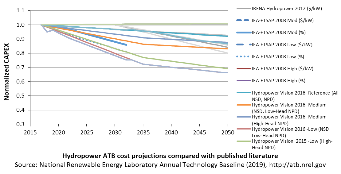
A range of literature projections is shown for comparison. The Mid and Low cost cases use a mix of inputs based on EIA technological learning assumptions, input from a technical team of Oak Ridge National Laboratory researchers, and the experience of expert hydropower consultants. Estimated 2035 cost levels are intended to provide order-of-magnitude cost reductions deemed to be at least conceptually possible, and they are meant to stimulate a broader discussion with the hydropower industry and its stakeholders that will be necessary to the future of cost reduction in the industry. Cost projections were derived independently for NPD and NSD technologies.
For context, ATB cost projections are compared to the literature, which represents 7 independent published studies and 11 cost projection scenarios within these studies. Cost reduction literature for hydropower is limited with several studies projecting no change through 2050. It is unclear whether (1) this represents a deliberate estimate of no future change in cost or (2) no estimate has been made.
Hydropower investment costs are very site specific and vary with type of technology. Literature was reviewed to attempt to isolate perceived CAPEX reduction for resources of similar characteristics over time (e.g., estimated cost to develop the same site in 2015, 2030, and 2050 based on different technology, installation, and other technical aspects). Some studies reflect increasing CAPEX over time. These studies were excluded from the ATB based on the interpretation that rising costs reflect a transition to less attractive sites as the better sites are used earlier.
Literature estimates generally reflect hydropower facilities of sizes similar to those represented in U.S. resource potential (i.e., they exclude estimates for very large facilities). Due to limited sample size, all projections are analyzed together without distinction between types of technology. Note that although declines are shown on a percentage basis, the reduction is likely to vary with initial capital cost. Large reductions for moderately expensive sites may not scale to more expensive sites or to less expensive sites. Projections derived for the Hydropower Vision study for different technologies (Low Head NPD, High Head NPD, and NSD) address this simplification somewhat.
Levelized Cost of Energy (LCOE) Projections
Levelized cost of energy (LCOE) is a summary metric that combines the primary technology cost and performance parameters: CAPEX, O&M, and capacity factor. It is included in the ATB for illustrative purposes. The ATB focuses on defining the primary cost and performance parameters for use in electric sector modeling or other analysis where more sophisticated comparisons among technologies are made. The LCOE accounts for the energy component of electric system planning and operation. The LCOE uses an annual average capacity factor when spreading costs over the anticipated energy generation. This annual capacity factor ignores specific operating behavior such as ramping, start-up, and shutdown that could be relevant for more detailed evaluations of generator cost and value. Electricity generation technologies have different capabilities to provide such services. For example, wind and PV are primarily energy service providers, while the other electricity generation technologies such as hydropower can provide capacity and flexibility services in addition to energy. These capacity and flexibility services are difficult to value and depend strongly on the system in which a new generation plant is introduced. These services are represented in electric sector models such as the ReEDS model and corresponding analysis results such as the Standard Scenarios.
The following three figures illustrate LCOE, which includes the combined impact of CAPEX, O&M, and capacity factor projections for hydropower across the range of resources present in the contiguous United States. For the purposes of the ATB, the costs associated with technology and project risk in the U.S. market are represented in the financing costs but not in the upfront capital costs (e.g., developer fees and contingencies). An individual technology may receive more favorable financing terms outside the United States, due to less technology and project risk, caused by more project development experience (e.g., offshore wind in Europe) or more government or market guarantees. The R&D Only LCOE sensitivity cases present the range of LCOE based on financial conditions that are held constant over time unless R&D affects them, and they reflect different levels of technology risk. This case excludes effects of tax reform, tax credits, and changing interest rates over time. The R&D + Market LCOE case adds to these financial assumptions: (1) the changes over time consistent with projections in the Annual Energy Outlook and (2) the effects of tax reform and tax credits. The representative plant characteristics in the ATB that best align with those of recently installed or anticipated near-term hydropower plants are associated with NPD 4. Data for all the resource categories can be found in the ATB Data spreadsheet; for simplicity, not all resource categories are shown in the figures.
R&D Only | R&D + Market
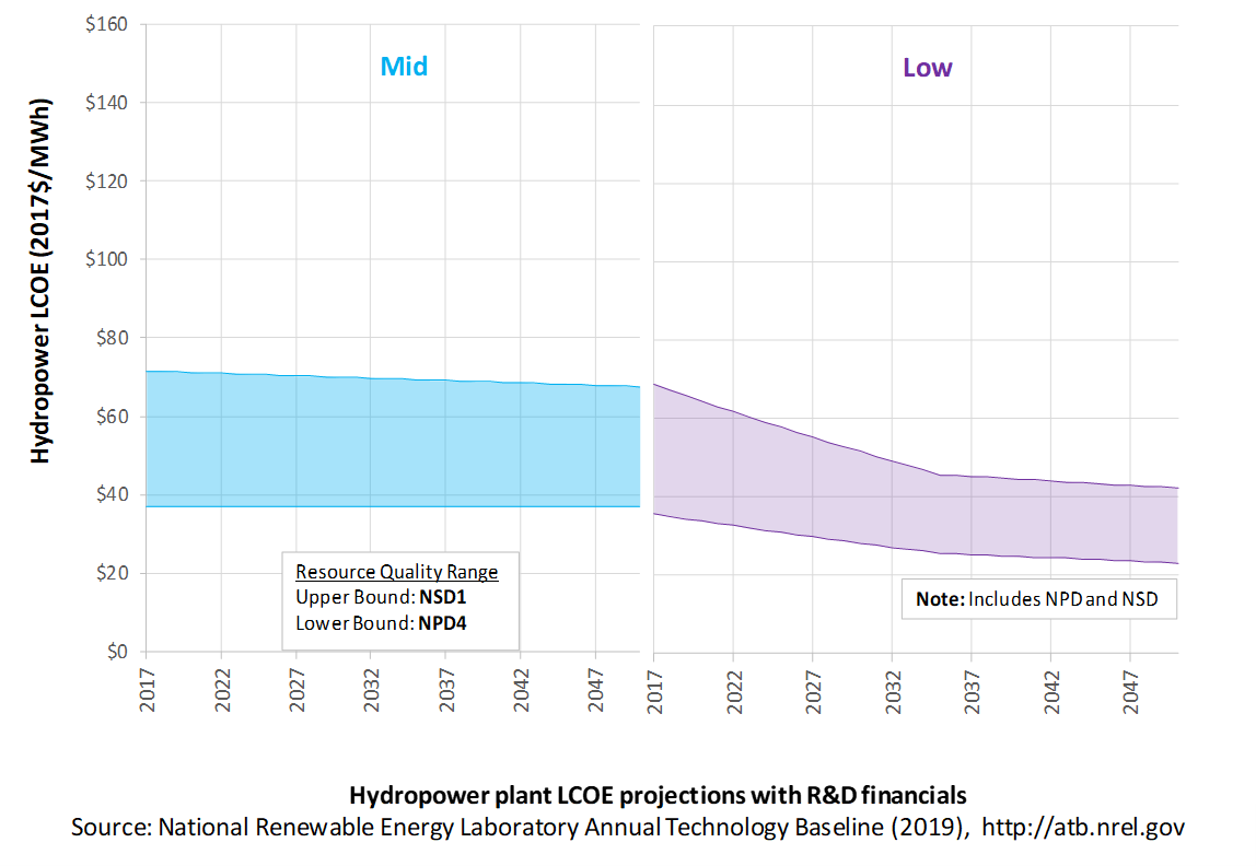
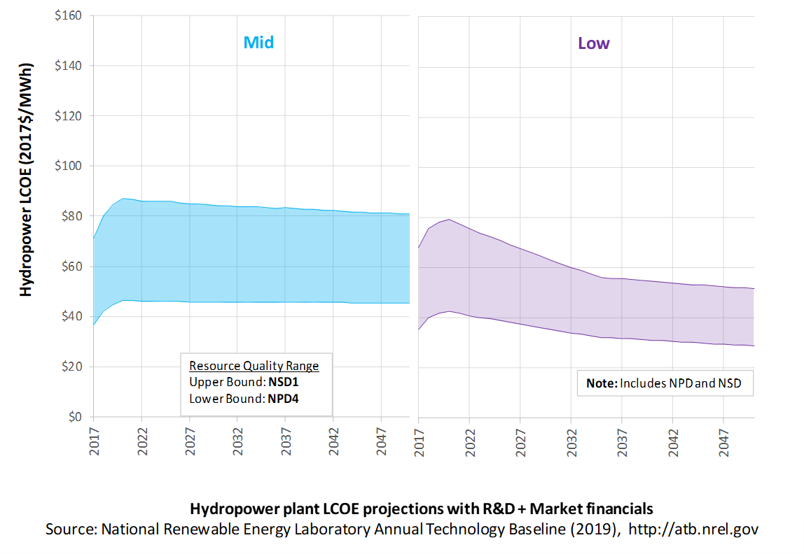
The methodology for representing the CAPEX, O&M, and capacity factor assumptions behind each pathway is discussed in Projections Methodology. In general, the degree of adoption of technology innovation distinguishes the Constant, Mid, and Low technology cost scenarios. These projections represent trends that reduce CAPEX and improve performance. Development of these scenarios involves technology-specific application of the following general definitions:
- Constant Technology: Base Year (or near-term estimates of projects under construction) equivalent through 2050 maintains current relative technology cost differences
- Mid Technology Cost Scenario: Technology advances through continued industry growth, public and private R&D investments, and market conditions relative to current levels that may be characterized as "likely" or "not surprising"
- Low Technology Cost Scenario: Technology advances that may occur with breakthroughs, increased public and private R&D investments, and/or other market conditions that lead to cost and performance levels that may be characterized as the " limit of surprise" but not necessarily the absolute low bound.
To estimate LCOE, assumptions about the cost of capital to finance electricity generation projects are required, and the LCOE calculations are sensitive to these financial assumptions. Two project finance structures are used within the ATB:
- R&D Only Financial Assumptions: This sensitivity case allows technology-specific changes to debt interest rates, return on equity rates, and debt fraction to reflect effects of R&D on technological risk perception, but it holds background rates constant at 2017 values from AEO2019 (EIA, 2019) and excludes effects of tax reform and tax credits.
- R&D Only + Market Financial Assumptions: This sensitivity case retains the technology-specific changes to debt interest, return on equity rates, and debt fraction from the R&D Only case and adds in the variation over time consistent with AEO2019 (EIA, 2019), as well as effects of tax reform and tax credits. For a detailed discussion of these assumptions, see Project Finance Impact on LCOE.
A constant cost recovery period – over which the initial capital investment is recovered – of 30 years is assumed for all technologies throughout this website, and can be varied in the ATB data spreadsheet.
The equations and variables used to estimate LCOE are defined on the Equations and Variables page. For illustration of the impact of changing financial structures such as WACC, see Project Finance Impact on LCOE. For LCOE estimates for the Constant, Mid, and Low technology cost scenarios for all technologies, see 2019 ATB Cost and Performance Summary.
In general, differences among the technology cost cases reflect different levels of adoption of innovations. Reductions in technology costs reflect the cost reduction opportunities that are listed below.
- Widespread implementation of value engineering and design/construction best practices
- Modular "drop-in" systems that minimize civil works and maximize ease of manufacture reduce both capital investment and O&M expenditures
- Use of alternative materials in place of steel for water diversion (e.g., penstocks)
- Implementation of standardized "smart" automation and remote monitoring systems to optimize scheduling of maintenance
- Research and development on environmentally enhanced turbines to improve performance of the existing hydropower fleet
- Efficient, certain, permitting, licensing, and approval procedures.
The Hydropower Vision study (DOE, 2016) includes road map actions that result in lower-cost technology.
Battery Storage
Energy storage technologies are important to document in the ATB because of their potential role in enhancing grid flexibility, especially under scenarios of high penetration of variable renewable technologies. CSP with TES and Hydropower both include storage capabilities, and a variety of other storage technologies could enhance the flexibility of the electrical grid. This section documents assumptions about only one of them: 4-hour, utility-scale, lithium-ion battery storage. NREL has completed recent analysis on ranges of costs related to other battery sizes (Fu, Remo, & Margolis, 2018) with relative costs represented in Figure ES-1 of the report (included below) which looked at 4-hour to 0.5 hour battery duration of utility scale plants.
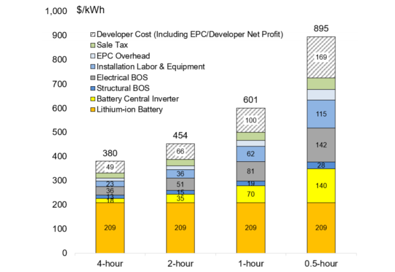
The ATB does not currently have costs for distributed battery storage-either for residential nor commercial applications behind the meter nor for a micro-grid or off-grid application. NREL has completed prior work on residential battery plus solar PV system analysis (Ardani et al., 2017) resulting in a range of costs of PV+battery systems as shown in the figure below. Note these costs are for 2016 and published in 2017, so we anticipate battery costs to be significantly lower currently.
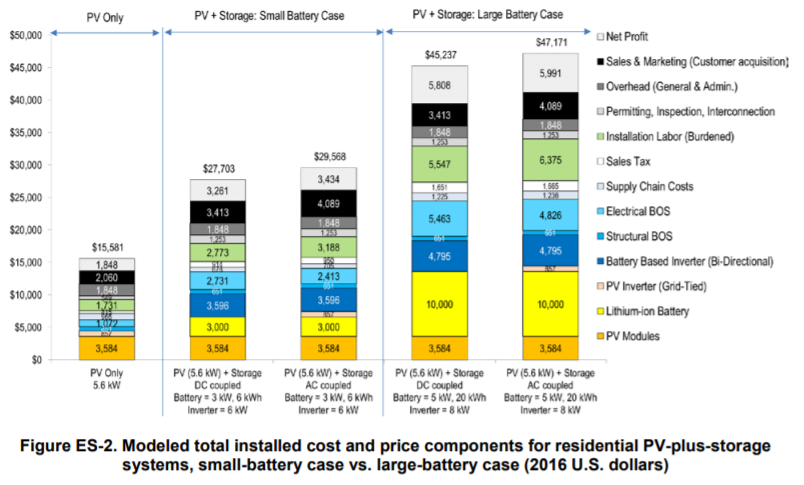
Base Year and Future Year Projections Overview
Battery cost and performance projections are based on a literature review of 25 sources published between 2016 and 2019, as described by Cole and Frazier (2019) . Three different projections from 2017 to 2050 were developed for scenario modeling based on this literature:
- High Technology Cost Scenario: generally based on the maximum of literature projections of future CAPEX and O&M technology pathway analysis; distinct from the Constant technology cost scenarios used among renewable energy technologies in the ATB
- Mid Technology Cost Scenario: generally based on the median of literature projections of future CAPEX and O&M technology pathway analysis
- Low Technology Cost Scenario: generally based on the low bound of literature projections of future CAPEX and O&M technology pathway analysis.
Standard Scenarios Model Results
ATB CAPEX, O&M, and round-trip efficiency assumptions for the Base Year and future projections through 2050 for High, Mid, and Low technology cost scenarios are used to develop the NREL Standard Scenarios using the ReEDS model. See ATB and Standard Scenarios.
Representative Technology
The representative technology was a utility-scale lithium-ion battery storage system with a 15-year life and a 4-hour rating, meaning it could discharge at its rated capacity for four hours as described by Cole and Frazier (2019) . Within the ATB spreadsheet, the costs are separated into energy and power cost estimates, which allow capital costs to be constructed for durations other than 4 hours according to the following equation:
For more information on the power vs. energy cost breakdown, see Cole and Frazier (2019) .
Capital Expenditures (CAPEX): Historical Trends, Current Estimates, and Future Projections
Recent Trends
Costs of lithium-ion battery storage systems have declined rapidly in recent years, prompting greater interest in utility-scale applications.
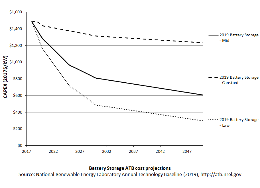
Base Year Estimates
The Base Year cost estimate is taken from Fu, Remo, and Margolis (2018). Comparisons to other reported costs for 2018 are included in Cole, Wesley & Frazier, A. Will (2019). Although the ATB uses a 2017 Base Year, the 2018 estimate based on the literature is the first year reported in the ATB, with a value of $1,484/kW in 2017 dollars.
Future Projections
Future projections are taken from Cole and Frazier (2019), which generally used the median of published cost estimates to develop a Mid Technology Cost Scenario and the minimum values to develop a Low Technology Cost Scenario. Analysts' judgment was used to select the long-term projections to 2050 from a sparse data set.
CAPEX Definition
The literature review does not enumerate elements of the capital cost of lithium-ion batteries (Cole, Wesley & Frazier, A. Will, 2019). However, the NREL storage cost report does detail a breakdown of capital costs with the actual battery pack being the largest component but significant other costs are also included. This breakdown is different if the battery is part of a hybrid system with solar PV. These relative costs for utility-scale standalone battery and battery + PV are demonstrated in the figure below (Fu, Remo, & Margolis, 2018).
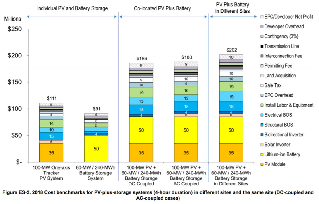
Operation and Maintenance (O&M) Costs
Base Year Estimates
Cole and Frazier (2019) assumed no variable operation and maintenance (VOM) cost. All operating costs were instead represented using fixed operation and maintenance (FOM) costs. The FOM costs include augmentation costs needed to keep the battery system operating at rated capacity for its lifetime. In the ATB, FOM is defined as the value needed to compensate for degradation to enable the battery system to have a constant capacity throughout its life. The literature review states that FOM costs are estimated at 2.5% of the $/kW capital costs.
Future Projections
In the ATB, the FOM cost remains constant at 2.5% of capital costs in all scenarios.
Round-trip efficiency is the ratio of useful energy output to useful energy input. Cole and Frazier (2019) identified 85% as a representative round-trip efficiency, and the ATB adopts this value.
Nuclear
The ATB includes a single nuclear power plant type. The cost and performance of this plant type is adapted from EIA data rather than derived from original analysis.
Capital Expenditures (CAPEX): Historical Trends, Current Estimates, and Future Projections
Nuclear power plant CAPEX is taken from the AEO2019 Reference Scenario (EIA, 2019a) with the adjustments discussed in the CAPEX definition section. The EIA advanced nuclear option is based on two AP1000 nuclear power plant units built on a brownfield site. The ATB includes only a single CAPEX projection for nuclear plants.
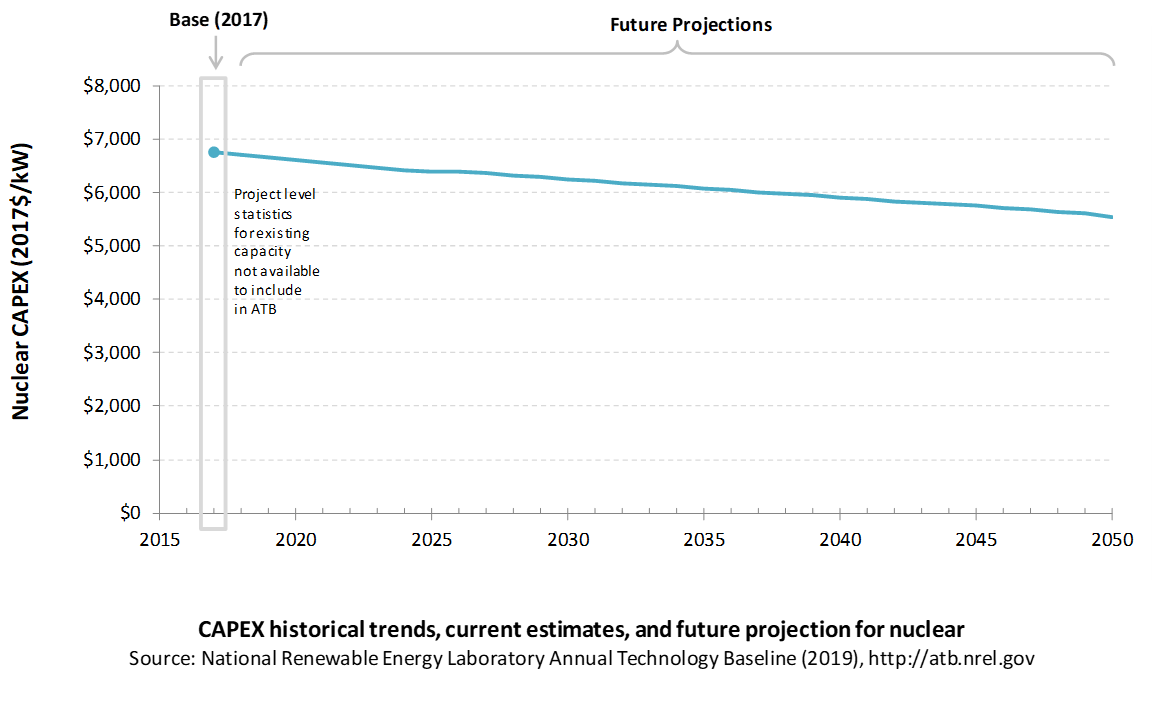
Comparison with Other Sources
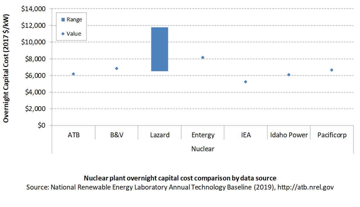
CAPEX Definition
Capital expenditures (CAPEX) are expenditures required to achieve commercial operation in a given year.
Overnight capital costs are modified from AEO2019 (EIA, 2019a). The EIA projections were adjusted by removing the material price index. The material price index accounts for projected changes in the price index for metals and metals products, and it is independent of the learning-based cost reductions applied in the EIA projections.
| Overnight Capital Cost ($/kW) | Construction Financing Factor (ConFinFactor) | CAPEX ($/kW) | |
| Nuclear: Advanced nuclear power generation | $6,200 | 1.087 | $6,742 |
CAPEX can be determined for a plant in a specific geographic location as follows:
Regional cost variations and geographically specific grid connection costs are not included in the ATB (CapRegMult = 1; GCC = 0). In the ATB, the input value is overnight capital cost (OCC) and details to calculate interest during construction (ConFinFactor).
In the ATB, CAPEX represents each type of nuclear plant with a unique value. Regional cost effects associated with labor rates, material costs, and other regional effects as defined by (EIA, 2016) expand the range of CAPEX (Plant × Region). Unique land-based spur line costs based on distance and transmission line costs are not estimated. The following figure illustrates the ATB representative plant relative to the range of CAPEX including regional costs across the contiguous United States. The ATB representative plants are associated with a regional multiplier of 1.0.
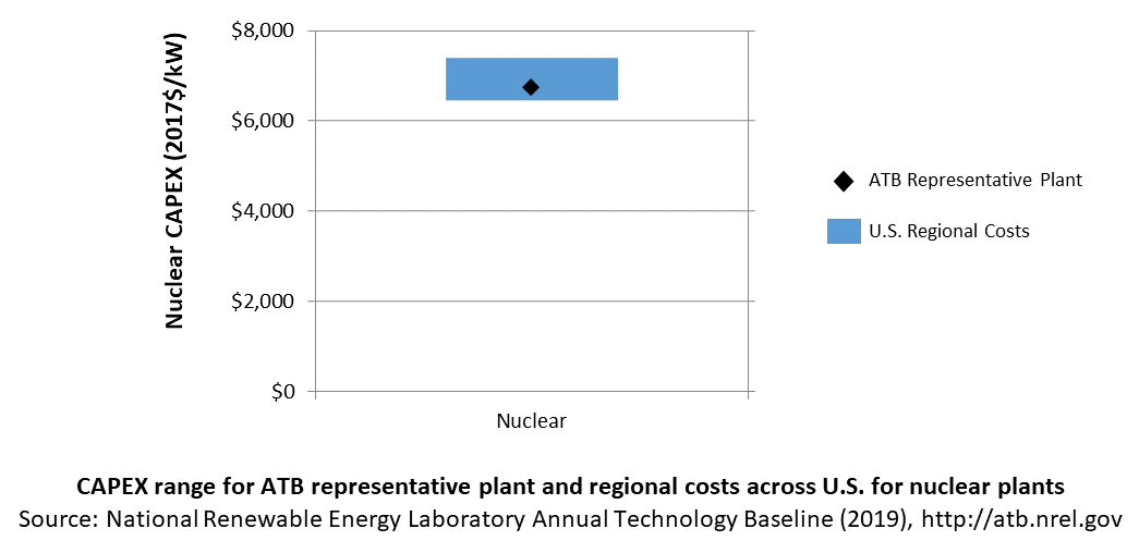
Operation and Maintenance (O&M) Costs
Nuclear power plant fixed and variable O&M costs are taken from table 8.2 of the AEO2019, and they are assumed to be constant over time.
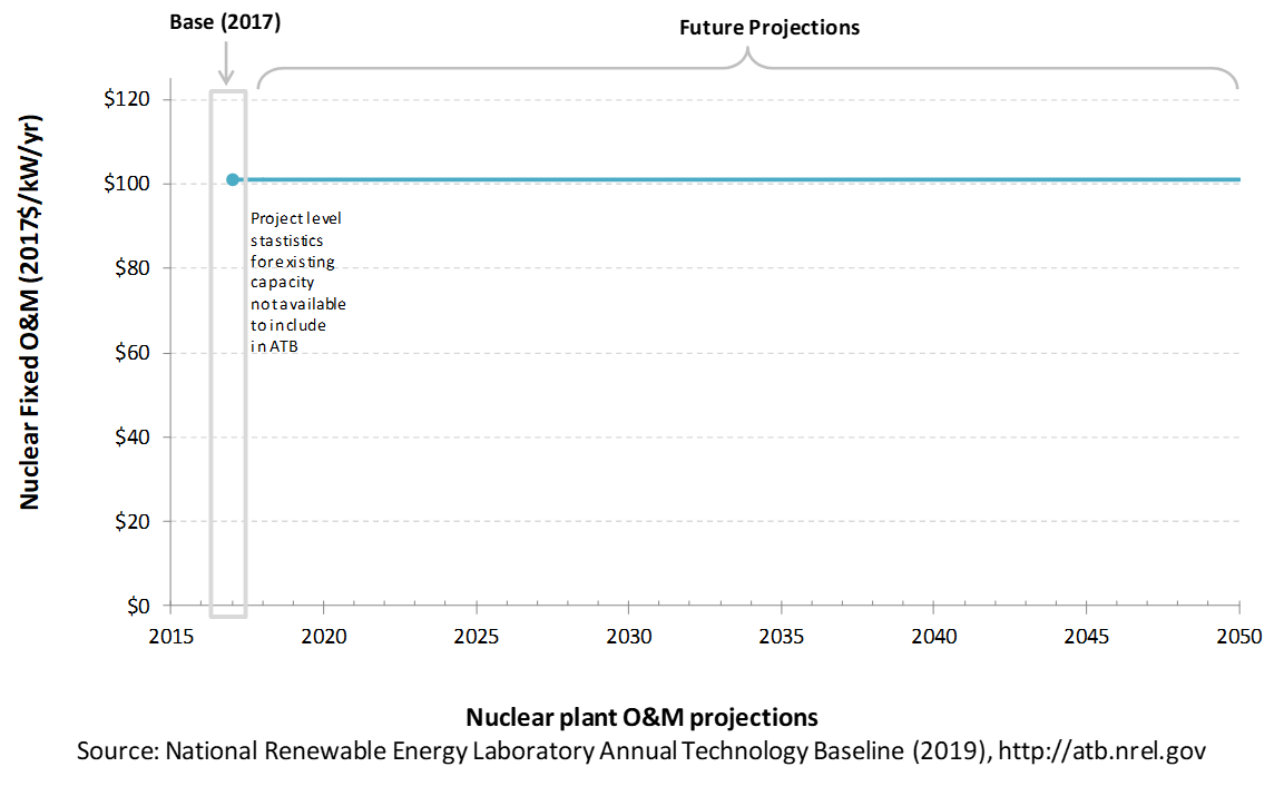
Capacity Factor: Expected Annual Average Energy Production Over Lifetime
The capacity factor represents the assumed annual energy production divided by the total possible annual energy production, assuming the plant operates at rated capacity for every hour of the year. For nuclear plants, the capacity factor is typically the same as (or very close to) their availability factor. For the ATB we assign the nuclear capacity factor as the fleet-wide average from 2017.
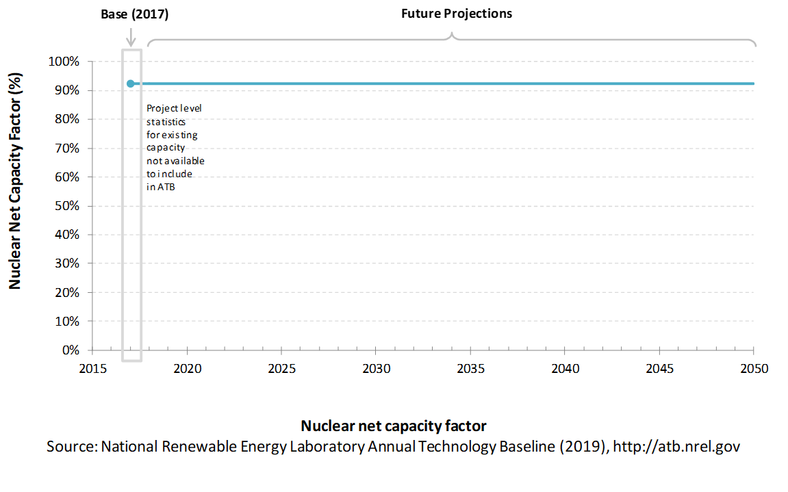
Levelized Cost of Energy (LCOE) Projections
Levelized cost of energy (LCOE) is a summary metric that combines the primary technology cost and performance parameters: CAPEX, O&M, and capacity factor. It is included in the ATB for illustrative purposes. The ATB focuses on defining the primary cost and performance parameters for use in electric sector modeling or other analysis where more sophisticated comparisons among technologies are made. The LCOE accounts for the energy component of electric system planning and operation. The LCOE uses an annual average capacity factor when spreading costs over the anticipated energy generation. This annual capacity factor ignores specific operating behavior such as ramping, start-up, and shutdown that could be relevant for more detailed evaluations of generator cost and value. Electricity generation technologies have different capabilities to provide such services. For example, wind and PV are primarily energy service providers, while the other electricity generation technologies provide capacity and flexibility services in addition to energy. These capacity and flexibility services are difficult to value and depend strongly on the system in which a new generation plant is introduced. These services are represented in electric sector models such as the ReEDS model and corresponding analysis results such as the Standard Scenarios.
The following three figures illustrate LCOE, which includes the combined impact of CAPEX, O&M, and capacity factor projections for nuclear across the range of resources present in the contiguous United States. For the purposes of the ATB, the costs associated with technology and project risk in the U.S. market are represented in the financing costs but not in the upfront capital costs (e.g., developer fees and contingencies). An individual technology may receive more favorable financing terms outside the United States, due to less technology and project risk, caused by more project development experience (e.g., offshore wind in Europe) or more government or market guarantees. The R&D Only LCOE sensitivity cases present the range of LCOE based on financial conditions that are held constant over time unless R&D affects them, and they reflect different levels of technology risk. This case excludes effects of tax reform, tax credits, and changing interest rates over time. The R&D + Market LCOE case adds to these financial assumptions: (1) the changes over time consistent with projections in the Annual Energy Outlook and (2) the effects of tax reform and tax credits.
R&D Only | R&D + Market
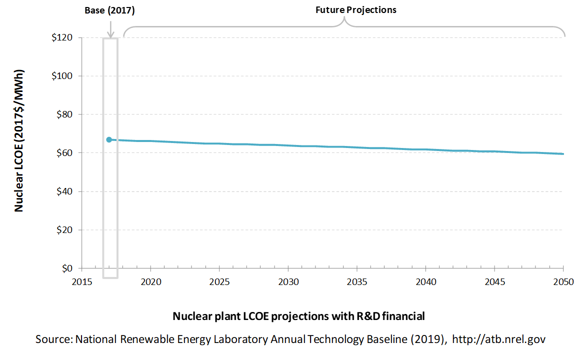

The LCOE of nuclear power plants is directly impacted by the cost of uranium, variations in the heat rate, and O&M costs, but the biggest factor is the capital cost (including financing costs) of the plant. The LCOE can also be impacted by the amount of downtime from refueling or maintenance. For a given year, the LCOE assumes that the fuel prices from that year continue throughout the lifetime of the plant.
Fuel prices are based on the AEO2019 (EIA, 2019a).
To estimate LCOE, assumptions about the cost of capital to finance electricity generation projects are required, and the LCOE calculations are sensitive to these financial assumptions. Two project finance structures are used within the ATB:
- R&D Only Financial Assumptions: This sensitivity case allows technology-specific changes to debt interest rates, return on equity rates, and debt fraction to reflect effects of R&D on technological risk perception, but it holds background rates constant at 2017 values from AEO2019 (EIA, 2019a) and excludes effects of tax reform and tax credits. A constant cost recovery period-or period over which the initial capital investment is recovered-of 30 years is assumed for all technologies.
- R&D Only + Market Financial Assumptions: This sensitivity case retains the technology-specific changes to debt interest, return on equity rates, and debt fraction from the R&D Only case and adds in the variation over time consistent with AEO2019 (EIA, 2019a) as well as effects of tax reform and tax credits. As in the R&D Only case, a constant cost recovery period-or period over which the initial capital investment is recovered-of 30 years is assumed for all technologies. For a detailed discussion of these assumptions, see Project Finance Impact on LCOE.
The equations and variables used to estimate LCOE are defined on the Equations and Variables page. For illustration of the impact of changing financial structures such as WACC, see Project Finance Impact on LCOE. For LCOE estimates for the Constant, Mid, and Low technology cost scenarios for all technologies, see 2019 ATB Cost and Performance Summary.
References
The following references are specific to this page; for all references in this ATB, see References.Ardani, K., O'Shaughnessy, E., Fu, R., McClurg, C., Huneycutt, J., & Margolis, R. (2017). Installed Cost Benchmarks and Deployment Barriers for Residential Solar Photovoltaics with Energy Storage: Q1 2016 (No. NREL/TP-7A40-67474). Retrieved from National Renewable Energy Laboratory website: Installed Cost Benchmarks and Deployment Barriers for Residential Solar Photovoltaics with Energy Storage: Q1 2016
Barbose, G., & Darghouth, N. (2018). Tracking the Sun XI: The Installed Price of Residential and Non-Residential Photovoltaic Systems in the United States (No. LBNL-2001062). https://doi.org/10.2172/1477384
Black & Veatch. (2012). Cost and Performance Data for Power Generation Technologies. Retrieved from Black & Veatch Corporation website: https://www.bv.com/docs/reports-studies/nrel-cost-report.pdf
Bolinger, M., & Seel, J. (2018). Utility-Scale Solar: An Empirical Trends in Project Technology, Cost, Performance, and PPA Pricing in the United States (2018 Edition). Retrieved from Lawrence Berkeley National Laboratory website: https://emp.lbl.gov/sites/default/files/lbnl_utility_scale_solar_2018_edition_report.pdf
Breyer, C., Afanasyeva, S., Brakemeier, D., Engelhard, M., Giuliano, S., Puppe, M., … Moser, M. (2017). Assessment of Mid-Term Growth Assumptions and Learning Rates for Comparative Studies of CSP and Hybrid PV-Battery Power Plants. AIP Conference Proceedings, 1850, 160001-1-160001–160009. https://doi.org/10.1063/1.4984535
Cole, W., Lewis, H., Sigrin, B., & Margolis, R. (2016). Interactions of Rooftop PV Deployment with the Capacity Expansion of the Bulk Power System. Applied Energy, 168, 473–481. https://doi.org/10.1016/j.apenergy.2016.02.004
Cole, Wesley, & Frazier, A. Will. (2019). Cost Projections for Utility-Scale Battery Storage (No. NREL/TP-6A20-73222). Retrieved from National Renewable Energy Laboratory website: https://www.nrel.gov/docs/fy19osti/73222.pdf
CSP Today Global Tracker. (n.d.). Retrieved February 11, 2019, from New Energy Update website: http://tracker.newenergyupdate.com/tracker/projects
Danko, P. (2015, February 10). SolarReserve: Crescent Dunes Solar Tower Will Power Up in March, Without Ivanpah's Woes. Retrieved February 5, 2019, from Breaking Energy website: https://breakingenergy.com/2015/02/10/solarreserve-crescent-dunes-solar-tower-will-power-up-in-march-without-ivanpahs-woes/
DOE. (2012). SunShot Vision Study. Retrieved from https://www1.eere.energy.gov/solar/pdfs/47927.pdf
DOE. (2016). Hydropower Vision: A New Chapter for America's Renewable Electricity Source (No. DOE/GO-102016-4869). Retrieved from U.S. Department of Energy website: https://www.energy.gov/sites/prod/files/2018/02/f49/Hydropower-Vision-021518.pdf
EERE. (n.d.). Goals of the Solar Energy Technologies Office. Retrieved March 16, 2019, from DOE Office of Energy Efficiency and Renewable Energy website: https://www.energy.gov/eere/solar/goals-solar-energy-technologies-office
EIA. (2016b). Capital Cost Estimates for Utility Scale Electricity Generating Plants. Retrieved from U.S. Energy Information Administration website: https://www.eia.gov/analysis/studies/powerplants/capitalcost/pdf/capcost_assumption.pdf
EIA. (2019a). Annual Energy Outlook 2019 with Projections to 2050. Retrieved from U.S. Energy Information Administration website: https://www.eia.gov/outlooks/aeo/pdf/AEO2019.pdf
Entergy Arkansas. (2015). 2015 Integrated Resource Plan. Retrieved from Entergy Arkansas, Inc. website: http://entergy-arkansas.com/content/transition_plan/IRP_Materials_Compiled.pdf
Feldman, D., & Margolis, R. (2018, November). Q2/Q3 2018 Solar Industry Update. Retrieved from https://www.nrel.gov/docs/fy19osti/72810.pdf
Feldman, D., Margolis, R., Denholm, P., & Stekli, J. (2016). Exploring the Potential Competitiveness of Utility-Scale Photovoltaics plus Batteries with Concentrating Solar Power, 2015-2030 (No. NREL/TP-6A20-66592). https://doi.org/10.2172/1321487
Fu, R., Feldman, D., & Margolis, R. (2018). U.S. Solar Photovoltaic System Cost Benchmark: Q1 2018. https://doi.org/10.2172/1484344
Fu, R., Remo, T. W., & Margolis, R. M. (2018). 2018 U.S. Utility-Scale Photovoltaics-Plus-Energy Storage System Costs Benchmark (No. NREL/TP-6A20-71714). https://doi.org/10.2172/1483474
Gagnon, P., Margolis, R., Melius, J., Phillips, C., & Elmore, R. (2016). Rooftop Solar Photovoltaic Technical Potential in the United States: A Detailed Assessment (No. NREL/TP-6A20-65298). https://doi.org/10.2172/1236153
IRENA. (2016b). The Power to Change: Solar and Wind Cost Reduction Potential to 2025. Retrieved from International Renewable Energy Agency website: https://www.irena.org/DocumentDownloads/Publications/IRENA_Power_to_Change_2016.pdf
IRENA. (2018). Renewable Power Generation Costs in 2017. Retrieved from International Renewable Energy Agency website: https://www.irena.org/-/media/Files/IRENA/Agency/Publication/2018/Jan/IRENA_2017_Power_Costs_2018.pdf
Kao, S.-C., McManamay, R. A., Stewart, K. M., Samu, N. M., Hadjerioua, B., DeNeale, S. T., … Smith, B. T. (2014). New Stream-Reach Development: A Comprehensive Assessment of Hydropower Energy Potential in the United States (No. ORNL/TM-2013/514). https://doi.org/10.2172/1130425
Kistner, R. (2016). Update on recent developments in the CSP technology. Retrieved from https://www.giz.de/de/downloads/giz2016_en_CSP%20Update_Abu%20Dhabi.pdf
Kurup, P., & Turchi, C. (2015). Parabolic Trough Collector Cost Update for the System Advisor Model (SAM) (No. NREL/TP-6A20-65228). https://doi.org/10.2172/1227713
Labastida, R. R., & Gauntlett, D. (2016). Next-Generation Solar PV: High Efficiency Solar PV Modules and Module-Level Power Electronics: Global Market Analysis and Forecasts [Market Report]. Chicago, IL: Navigant Research.
Lazard. (2016). Lazard's Levelized Cost of Energy Analysis: Version 10.0. Retrieved from Lazard website: https://www.lazard.com/media/438038/levelized-cost-of-energy-v100.pdf
Lilliestam, J., Labordena, M., Patt, A., & Pfenninger, S. (2017). Empirically Observed Learning Rates for Concentrating Solar Power and their Responses to Regime Change. Nature Energy, 2(7), 17094. https://doi.org/10.1038/nenergy.2017.94
Lopez, A., Roberts, B., Heimiller, D., Blair, N., & Porro, G. (2012). U.S. Renewable Energy Technical Potentials: A GIS-Based Analysis (Technical Report No. NREL/TP-6A20-51946). https://doi.org/10.2172/1219777
Mehos, M., Kabel, D., & Smithers, P. (2009). Planting the Seed: Greening the Grid with Concentrating Solar Power. IEEE Power and Energy Magazine, 7(3), 55–62. https://doi.org/10.1109/MPE.2009.932308
Mehos, M., Turchi, C., Vidal, J., Wagner, M., & Ma, Z. (2017). Concentrating Solar Power Gen3 Demonstration Roadmap (No. NREL/TP-5500-67464). https://doi.org/10.2172/1338899
Murphy, C., Sun, Y., Cole, W., Maclaurin, G., Turchi, C., & Mehos, M. (2019). The Potential Role of Concentrating Solar Power Within the Context of DOE's 2030 Solar Cost Targets (No. NREL/TP-6A20-71912). https://doi.org/10.2172/1491726
MWH. (2009). Hydropower Modernization Initiative, Phase I, Needs and Opportunities Evaluation and Ranking (No. Contract No. W9127N-08-D-0003. Task Order 001.). Montgomery Watson Harza.
NREL, & SolarPaces. (n.d.). Concentrating Solar Power Projects. Retrieved February 11, 2019, from https://solarpaces.nrel.gov/
NREL. (n.d.a). National Solar Radiation Database (NSRDB) Data Viewer. Retrieved March 17, 2019, from NREL Geospatial Data Science Data and Tools website: https://maps.nrel.gov/nsrdb-viewer/?aL=f69KzE%255Bv%255D%3Dt&bL=H7Qphn&cE=0&lR=f69KzE.0%255Ba%255D%3Df%26f69KzE.1%255Ba%255D%3Df%26f69KzE.2%255Ba%255D%3Df%26f69KzE.3%255Ba%255D%3Df%26f69KzE.4%255Ba%255D%3Df%26f69KzE.5%255Ba%255D%3Df%26f69KzE.7%255Ba%255D%3Df%26f69KzE.8%255Ba%255D%3Df&mC=33.92626920481366%2C-110.75248718261719&zL=12
NREL. (n.d.b). System Advisor Model (SAM). Retrieved January 26, 2018, from National Renewable Energy Laboratory website: https://sam.nrel.gov/
O'Connor, P. W., Zhang, Q. F. (Katherine), DeNeale, S. T., Chalise, D. R., & Centurion, E. E. (2015). Hydropower Baseline Cost Modeling (No. ORNL/TM-2015/14). https://doi.org/10.2172/1185882
Roberts, B. J. (2018). Map of solar resource in contiguous United States. Retrieved from https://www.nrel.gov/gis/assets/pdfs/solar_dni_2018_01.pdf
Shemer, N. (2018, April 16). CSP capex costs fall by almost half as developers shift towards China and Middle East. Retrieved April 24, 2019, from http://newenergyupdate.com/csp-today/csp-capex-costs-fall-almost-half-developers-shift-towards-china-and-middle-east
SolarReserve. (n.d.). Sandstone (project overview). Retrieved February 11, 2019, from SolarReserve website: https://www.solarreserve.com/en/global-projects/csp/sandstone
Taylor, P. (2016, March 29). Nev. Plant Solves Quandary of How to Store Sunshine. E&E Greenwire. Retrieved from https://www.eenews.net/stories/1060034748
Turchi, C. (2010). Parabolic Trough Reference Plant for Cost Modeling with the Solar Advisor Model (SAM) (No. NREL/TP-550-47605). https://doi.org/10.2172/983729
Turchi, Craig, & Heath, G. (2013). Molten Salt Power Tower Cost Model for the System Advisor Model (SAM) (No. NREL/TP-5500-57625). https://doi.org/10.2172/1067902
Turchi, Craig, Boyd, M., Kesseli, D., Kurup, P., Mehos, M., Neises, T., … Wendelin, T. (2019). CSP Systems Analysis - Final Project Report (No. NREL/TP-5500-72856). Retrieved from National Renewable Energy Laboratory website: https://www.nrel.gov/docs/fy19osti/72856.pdf
Varro, L., & Ha, J. (2015). Projected Costs of Generating Electricity: 2015 Edition. Retrieved from International Energy Agency website: https://www.iea.org/media/presentations/150831_ProjectedCostsOfGeneratingElectricity_Presentation.pdf
World Bank. (2014). Project Appraisal Document on a Proposed Loan in the Amount of EUR234.50 Million and US$80 Million (US$400 Million Equivalent) and a Proposed Loan from the Clean Technology Fund in the Amount of US$119 Million to the Moroccan Agency for Solar Energy with Guarantee from the Kingdom of Morocco for the Noor-Ouarzazate Concentrated Solar Power Plant Project (No. PAD1007). Retrieved from The World Bank website: http://documents.worldbank.org/curated/en/748641468279941398/pdf/PAD10070PAD0P100disclosed0120220140.pdf