Annual Technology Baseline 2017
National Renewable Energy Laboratory
Recommended Citation:
NREL (National Renewable Energy Laboratory). 2017. 2017 Annual Technology Baseline. Golden, CO: National Renewable Energy Laboratory. http://atb.nrel.gov/.
Please consult Guidelines for Using ATB Data:
https://atb.nrel.gov/electricity/user-guidance.html
2017 ATB
For each electricity generation technology in the ATB, this website provides:
- Capital expenditures (CAPEX): the definition of CAPEX used in the ATB and the historical trends, current estimates, and future projections of CAPEX used in the ATB
- Operations and maintenance (O&M) costs: the definition of O&M and the current estimates and future projections of O&M used in the ATB
- Capacity factor (CF): the definition of CF and the historical trends, current estimates, and future projections of CF used in the ATB
- Future cost and performance methods: an outline of the methodology used to make the projections of future cost and performance in the ATB for High, Mid, and Low cost cases
- Levelized cost of energy (LCOE): metric that combines CAPEX, O&M, CF, and projections for High-, Mid-, Low-cost cases for illustration of the combined effect of the primary cost and performance components and discussion of technology advances that yield future projections.
Electricity generation technologies are selected on the left side of the screen, and the topics highlighted above can be selected using the drop-down menu at the top-right of the screen.
Guidelines for using and interpreting ATB content are provided. LCOE captures the energy component of electric system planning and operation, but the electric system also requires capacity and flexibility services to operate reliably. These services are represented in electric sector models such as the Regional Energy Deployment Systems (ReEDS) model and corresponding analysis results such as the NREL Standard Scenarios.
The NREL Standard Scenarios, a companion product to the ATB, provides a suite of electric sector scenarios and associated assumptions—including technology cost and performance assumptions from the ATB.
ATB data sources and references are also provided for each technology. All dollar values are presented in 2015 U.S. dollars, unless noted otherwise.
Additional information about the 2017 ATB—available via links in the ATB website footer below—includes:
Geothermal
Hydrothermal Geothermal
Representative Technology
The typical geothermal plant size for hydrothermal resource sites is represented by a range of 30–40 MW, depending on the technology type (e.g., binary or flash) (Mines 2013).
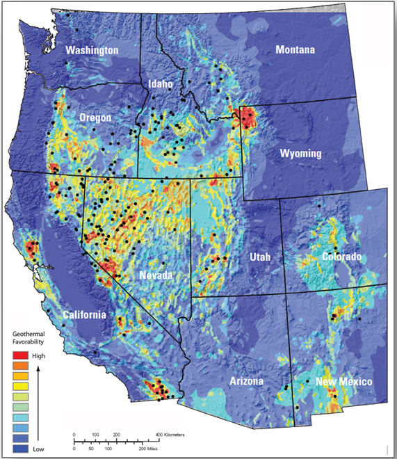
Resource Potential
The hydrothermal geothermal resource is concentrated in the western United States. The total potential is 45,370 MW: 7,833 MW identified and 37,537 MW undiscovered (Williams et al. 2008). The U.S. Geological Survey (Williams et al. 2008) identified resource potential at each site is based on available reservoir thermal energy information from studies conducted at the site. The undiscovered hydrothermal technical potential estimate is based on a series of GIS statistical models for the spatial correlation of geological factors that facilitate the formation of geothermal systems.
The U.S. Geological Survey resource potential estimates for hydrothermal were used with the following modifications:
- Installed capacity of about 3 GW in 2014 is excluded from the resource potential
- Technical potential estimates increased 20%–30% to reflect impact of in-field enhanced geothermal system (EGS) technologies to increase (1) productivity of dry wells and (2) recovery of heat in place from hydrothermal reservoirs.
Renewable energy technical potential, as defined by Lopez et al. (2012), represents the achievable energy generation of a particular technology given system performance, topographic limitations, and environmental and land-use constraints. The primary benefit of assessing technical potential is that it establishes an upper-boundary estimate of development potential. It is important to understand that there are multiple types of potential-resource, technical, economic, and market (Lopez et al. 2012; NREL, "Renewable Energy Technical Potential").
Base Year and Future Year Projections Overview
The Base Year cost and performance estimates are calculated using Geothermal Electricity Technology Evaluation Model (GETEM), a bottom-up cost analysis tool that accounts for each phase of development of a geothermal plant (DOE "Geothermal Electricity Technology Evaluation Model").
- Cost and performance data for hydrothermal generation plants are estimated for each potential site using GETEM. Model results are based on resource attributes (e.g., estimated reservoir temperature, depth, and potential) of each site.
- Site attribute values are from Williams et al. (2008) for identified resource potential and from capacity-weighted averages of site attribute values of nearby identified resources for undiscovered resource potential.
- GETEM is used to estimate CAPEX, O&M, and parasitic plant losses that affect net energy production.
Projections of CAPEX for plants installed in future years are derived from minimum learning estimates (IEA 2017). Capacity factor and O&M costs for plants installed in future years are unchanged from the Base Year. Projections for hydrothermal and EGS technologies are equivalent.
- High cost: no change in CAPEX, O&M, or capacity factor from 2015 to 2050; consistent across all renewable energy technologies in the ATB
- Mid cost: CAPEX cost reduction based on half of assumed minimum learning
- Low cost: CAPEX cost reduction based on assumed minimum learning.
Enhanced Geothermal System (EGS) Technology
Representative Technology
The typical geothermal plant size for EGS plants is represented by a range of 20-25 MW for binary or flash technologies (Mines 2013).
Resource Potential
The enhanced geothermal system (EGS) resource is concentrated in the western United States. The total potential is greater than 100,000 MW: 1,493 MW of near-hydrothermal field EGS (NF-EGS) and the remaining potential comes from deep EGS.
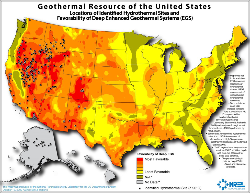
- The NF-EGS resource potential is based on data from USGS for EGS potential on the periphery of select studied and identified hydrothermal sites.
- The deep EGS resource potential (Augustine 2011) is based on Southern Methodist University Geothermal Laboratory temp-at-depth maps and the methodology is from MIT (2006).
- The EGS resource is thousands of GW (16,000 GW) but many locations are likely not commercially feasible.
Renewable energy technical potential as defined by Lopez et al., (2012) represents the achievable energy generation of a particular technology given system performance, topographic limitations, environmental, and land-use constraints. The primary benefit of assessing technical potential is that it establishes an upper-boundary estimate of development potential. It is important to understand that there are multiple types of potential-resource, technical, economic, and market (Lopez et al. 2012; NREL, "Renewable Energy Technical Potential").
Base Year and Future Projections Overview
The Base Year cost and performance estimates are calculated using the Geothermal Electricity Technology Evaluation Model (GETEM), a bottom-up cost analysis tool that accounts for each phase of development of a geothermal plant (DOE "Geothermal Electricity Technology Evaluation Model").
- Cost and performance data for EGS generation plants are estimated for each potential site using GETEM. Model results based on resource attributes (e.g., estimated reservoir temperature, depth, and potential) of each site.
- Approaches to restrict resource potential to about 500 GW based on USGS analysis may be implemented in the future.
- GETEM is used to estimate CAPEX and O&M. and parasitic plant losses that affect net energy production.
Projections of CAPEX for plants installed in future years are derived from minimum learning estimates (IEA 2017). Capacity factor and O&M costs for plants installed in future years are unchanged from the Base Year. Projections for hydrothermal and enhanced geothermal system technologies are equivalent.
- High Cost: no change in CAPEX, O&M, or capacity factor from 2015 to 2050, consistent across all renewable energy technologies in the ATB
- Mid Cost: CAPEX cost reduction based on half of assumed minimum learning
- Low cost: CAPEX cost reduction based on assumed minimum learning.
CAPital EXpenditures (CAPEX): Historical Trends, Current Estimates, and Future Projections
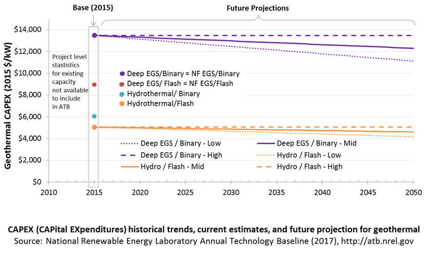
Capital expenditures (CAPEX) are expenditures required to achieve commercial operation in a given year. These expenditures include the geothermal generation plant, the balance of system (e.g., site preparation, installation, and electrical infrastructure), and financial costs (e.g., development costs, onsite electrical equipment, and interest during construction) and are detailed in CAPEX Definition. In the ATB, CAPEX reflects typical plants and does not include differences in regional costs associated with labor or materials. The range of CAPEX demonstrates variation with resource in the contiguous United States.
The following figure shows the Base Year estimate and future year projections for CAPEX costs. Three cost reduction scenarios are represented: High, Mid, and Low. The estimate for a given year represents CAPEX of a new plant that reaches commercial operation in that year.
Base Year Estimates
For illustration in the ATB, six representative geothermal plants are shown. Two energy conversion processes are common: binary organic Rankine cycle and flash.
- Binary plants use a heat exchanger to transfer geothermal energy to an organic Rankine cycle. This technology generally applies to lower-temperature systems. These systems have higher CAPEX than flash systems because of the increased number of components, their lower-temperature operation, and a general requirement that a number of wells be drilled for a given power output.
- Flash plants create steam directly from the thermal fluid through a pressure change. This technology generally applies to higher-temperature systems. Due to the reduced number of components and higher-temperature operation, these systems generally produce more power per well, thus reducing drilling costs. These systems generally have lower CAPEX than binary systems.
Examples using each of these plant types in each of the three resource types (hydrothermal, NF-EGS, and deep EGS) are shown in the ATB.
Costs are for new or "greenfield" hydrothermal projects, not for re-drilling or additional development/capacity additions at an existing site.
Characteristics for the six example plants representing current technology were developed based on discussion with industry stakeholders. The CAPEX estimates were generated using GETEM. CAPEX for NF-EGS and EGS are equivalent.
The table below shows the range of OCC associated with the resource characteristics for potential sites throughout the United States.
| Temp (°C) | |||||
|---|---|---|---|---|---|
| >=200C | 150–200 | 135–150 | <135 | ||
| Hydrothermal | |||||
| Number of identified sites | 21 | 23 | 17 | 59 | |
| Total capacity (MW) | 22,718 | 5,560 | 1,173 | 9,697 | |
| Avgerage OCC ($/kW) | 4,047 | 6,801 | 8,611 | 15,367 | |
| Min. OCC ($/kW) | 3,000 | 3,909 | 6,786 | 10,596 | |
| Max. OCC ($/kW) | 5,906 | 15,314 | 11,885 | 20,612 | |
| Example plant OCC ($/kW) | 4,567 | 5,465 | |||
| NF-EGS | Number of sites | 12 | 20 | ||
| Total capacity (MW) | 787 | 707 | |||
| Avgerage OCC ($/kW) | 5,928 | 8,820 | |||
| Min. OCC ($/kW) | 4,871 | 6,757 | |||
| Max. OCC ($/kW) | 7,216 | 11,486 | |||
| Example plant OCC ($/kW) | 8,100 | 12,179 | |||
| Deep EGS (3–6 km) | Number of sites | n/a | n/a | ||
| Total capacity (MW) | 100,000+ | ||||
| Average OCC ($/kW) | 10,061 | 20,840 | |||
| Min.OCC ($/kW) | 4,782 | 15,951 | |||
| Max. OCC ($/kW) | 18,292 | 25,933 | |||
| Example plant OCC ($/kW) | 8,100 | 12,179 | |||
Future Year Projections
Projection of future geothermal plant CAPEX for the Low case is based on minimum learning rates as implemented in AEO (EIA 2015): 10% by 2035. This corresponds to a 0.5% annual improvement in CAPEX, which is assumed to continue on through 2050. The Mid case is also considered with a 0.25% annual improvement in CAPEX through 2050.
A detailed description of the methodology for developing Future Year Projections is found in Projections Methodology.
Technology innovations that could impact future CAPEX costs are summarized in LCOE Projections.
CAPEX Definition
Capital expenditures (CAPEX) are expenditures required to achieve commercial operation in a given year.
For the ATB - and based on EIA (2016a) and GETEM component cost calculations - the geothermal plant envelope is defined to include:
- Geothermal generation plant
- Exploration, confirmation drilling, well field development, reservoir stimulation (EGS), plant equipment, and plant construction
- Power plant equipment, well-field equipment, and components for wells (including dry/non-commercial wells)
- Balance of system (BOS)
- Installation and electrical infrastructure, such as transformers, switchgear, and electrical system connecting turbines to each other and to the control center
- Project indirect costs, including costs related to engineering, distributable labor and materials, construction management start up and commissioning, and contractor overhead costs, fees, and profit
- Financial costs
- Owner's costs, such as development costs, preliminary feasibility and engineering studies, environmental studies and permitting, legal fees, insurance costs, and property taxes during construction
- Electrical interconnection and onsite electrical equipment (e.g., switchyard), a nominal-distance spur line (<1 mile), and necessary upgrades at a transmission substation; distance-based spur line cost (GCC) not included in the ATB
- Interest during construction estimated based on four-year duration accumulated 10%/20%/30%/40% at half-year intervals and an 8% interest rate (ConFinFactor).
CAPEX can be determined for a plant in a specific geographic location as follows:
CAPEX = ConFinFactor*(OCC*CapRegMult+GCC).
(See the Financial Definitions tab in the ATB data spreadsheet.)
Regional cost variations and geographically specific grid connection costs are not included in the ATB (CapRegMult = 1; GCC = 0). In the ATB, the input value is overnight capital cost (OCC) and details to calculate interest during construction (ConFinFactor).
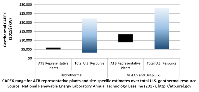
In the ATB, CAPEX is shown for six representative plants. Example CAPEX for binary organic Rankine cycle and flash energy conversion processes in each of three geothermal resource types are presented. CAPEX estimates for all hydrothermal NF-EGS potential results in a CAPEX range that is much broader than that shown in the ATB. It is unlikely that all of the resource potential will be developed due to the very high costs for some sites. Regional cost effects and distance-based spur line costs are not estimated.
Standard Scenarios Model Results
ATB CAPEX, O&M, and capacity factor assumptions for the Base Year and future projections through 2050 for High, Mid, and Low projections are used to develop the NREL Standard Scenarios using the ReEDS model. See ATB and Standard Scenarios.
The ReEDS model represents cost and performance for hydrothermal, NF-EGS, and EGS potential in 5 bins for each of 134 geographic regions, resulting in a greater CAPEX range in the reference supply curve than what is shown in examples in the ATB.
CAPEX in the ATB does not represent regional variants (CapRegMult) associated with labor rates, material costs, etc., and neither does the ReEDS model.
CAPEX in the ATB does not include geographically determined spur line (GCC) from plant to transmission grid, and neither does the ReEDS model.
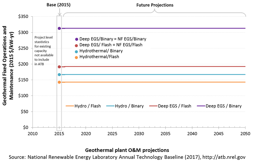
Operation and Maintenance (O&M) Costs
Operations and maintenance (O&M) costs represent average annual fixed expenditures (and depend on rated capacity) required to operate and maintain a hydrothermal plant over its technical lifetime of 30 years (plant and reservoir) (the distinction between economic life and technical life is described here), including:
- Insurance, taxes, land lease payments, and other fixed costs
- Present value and annualized large component overhaul or replacement costs over technical life (e.g., downhole pumps)
- Scheduled and unscheduled maintenance of geothermal plant components and well field components over the technical lifetime of the plant and reservoir.
The following figure shows the Base Year estimate and future year projections for fixed O&M (FOM) costs. Three cost reduction scenarios are represented. The estimate for a given year represents annual average FOM costs expected over the technical lifetime of a new plant that reaches commercial operation in that year.
Base Year Estimates
FOM is estimated for each example plant based on technical characteristics.
GETEM is used to estimate FOM for each of the six representative plants. FOM for NF-EGS and EGS are equivalent.
Future Year Projections
No future FOM cost reduction is assumed in this edition of the ATB.
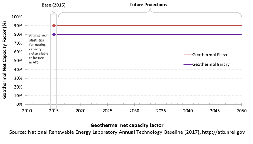
Capacity Factor: Expected Annual Average Energy Production Over Lifetime
The capacity factor represents the expected annual average energy production divided by the annual energy production, assuming the plant operates at rated capacity for every hour of the year. It is intended to represent a long-term average over the technical lifetime of the plant (the distinction between economic life and technical life is described here). It does not represent interannual variation in energy production. Future year estimates represent the estimated annual average capacity factor over the technical lifetime of a new plant installed in a given year.
Geothermal plant capacity factor is influenced by diurnal and seasonal air temperature variation (for air-cooled plants), technology (e.g., binary or flash), downtime, and internal plant energy losses.
The following figure shows a range of capacity factors based on variation in the resource for plants in the contiguous United States. The range of the Base Year estimates illustrates Binary or Flash geothermal plants. Future year projections for High, Mid, and Low cost scenarios are unchanged from the Base Year. Technology improvements are focused on CAPEX cost elements.
Base Year Estimate
The capacity factor estimates are developed using GETEM at typical design air temperature and based on design plant capacity net losses. An additional reduction is applied to approximate potential variability due to seasonal temperature effects.
Some geothermal plants have experienced year-on-year reductions in energy production, but this is not consistent across all plants. No approximation of long-term degradation of energy output is assumed.
Ongoing work at NREL and the Idaho National Laboratory is helping improve capacity factor estimates for geothermal plants. As this work progresses, it will be incorporated into future versions of the ATB.
Future Year Projections
Capacity factors remain unchanged from the Base Year through 2050. Technology improvements are focused on CAPEX costs. Estimates of capacity factor for geothermal plants in the ATB represent typical operation. The dispatch characteristics of these systems are valuable to the electric system to manage changes in net electricity demand. Actual capacity factors will be influenced by the degree to which system operators call on geothermal plants to manage grid services.
Plant Cost and Performance Projections Methodology
The site-specific nature of geothermal plant cost, the relative maturity of hydrothermal plant technology, and the very early stage development of EGS technologies make cost projections difficult. No thorough literature reviews have been conducted for cost reduction of hydrothermal geothermal technologies or EGS technologies. However, the Geothermal Vision Study, which is sponsored by the DOE Geothermal Technologies Office, is currently underway and is likely to lead to industry-developed cost reduction estimates that could be included in a future ATB..
Projection of future geothermal plant CAPEX for the Low cost case is based on minimum learning rates as implemented in AEO (EIA 2015): 10% by 2035. This corresponds to a 0.5% annual improvement in CAPEX, which is assumed to continue on through 2050. The Mid cost case assumes a 0.25% annual improvement in CAPEX through 2050. The High cost case retains all cost and performance assumptions equivalent to the Base Year through 2050.
Levelized Cost of Energy (LCOE) Projections
Levelized cost of energy (LCOE) is a simple metric that combines the primary technology cost and performance parameters, CAPEX, O&M, and capacity factor. It is included in the ATB for illustrative purposes. The focus of the ATB is to define the primary cost and performance parameters for use in electric sector modeling or other analysis where more sophisticated comparisons among technologies are made. LCOE captures the energy component of electric system planning and operation, but the electric system also requires capacity and flexibility services to operate reliably. Electricity generation technologies have different capabilities to provide such services. For example, wind and PV are primarily energy service providers, while the other electricity generation technologies provide capacity and flexibility services in addition to energy. These capacity and flexibility services are difficult to value and depend strongly on the system in which a new generation plant is introduced. These services are represented in electric sector models such as the ReEDS model and corresponding analysis results such as the Standard Scenarios.
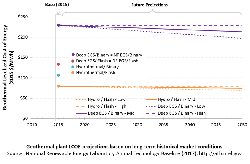
The following three figures illustrate the combined impact of CAPEX, O&M, and capacity factor projections across the range of resources present in the contiguous United States. The Current Market Conditions LCOE demonstrates the range of LCOE based on macroeconomic conditions similar to the present. The Historical Market Conditions LCOE presents the range of LCOE based on macroeconomic conditions consistent with prior ATB editions and Standard Scenarios model results. The Normalized LCOE (all LCOE estimates are normalized with the lowest Base Year LCOE value) emphasizes the effect of resource quality and the relative differences in the three future pathways independent of project finance assumptions. The ATB representative plant characteristics that best align with recently installed or anticipated near-term geothermal plants are associated with Hydrothermal/Flash. Data for all the resource categories can be found in the ATB data spreadsheet.
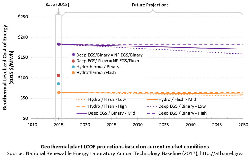
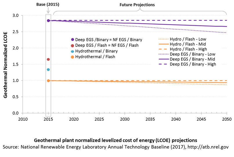
The methodology for representing the CAPEX, O&M, and capacity factor assumptions behind each pathway is discussed in Projections Methodology. The three pathways are generally defined as:
- High = Base Year (or near-term estimates of projects under construction) equivalent through 2050 maintains current relative technology cost differences
- Mid = Technology advances through continued industry growth, public and private R&D investments, and market conditions relative to current levels that may be characterized as "likely" or "not surprising"
- Low = Technology advances that may occur with breakthroughs, increased public and private R&D investments, and/or other market conditions that lead to cost and performance levels that may be characterized as the "limit of surprise" but not necessarily the absolute low bound.
To estimate LCOE, assumptions about the cost of capital to finance electricity generation projects are required. For comparison in the ATB, two project finance structures are represented.
- Current Market Conditions: The values of the production tax credit (PTC) and investment tax credit (ITC) are ramping down by 2020, at which time wind and solar projects may be financed with debt fractions similar to other technologies. This scenario reflects debt interest (4.4% nominal, 1.9% real) and return on equity rates (9.5% nominal, 6.8% real) to represent 2017 market conditions (AEO 2017) and a debt fraction of 60% for all electricity generation technologies. An economic life, or period over which the initial capital investment is recovered, of 20 years is assumed for all technologies. These assumptions are one of the project finance options in the ATB spreadsheet.
- Long-Term Historical Market Conditions: Historically, debt interest and return on equity were represented with higher values. This scenario reflects debt interest (8% nominal, 5.4% real) and return on equity rates (13% nominal, 10.2% real) implemented in the ReEDS model and reflected in prior versions of the ATB and Standard Scenarios model results. A debt fraction of 60% for all electricity generation technologies is assumed. An economic life, or period over which the initial capital investment is recovered, of 20 years is assumed for all technologies. These assumptions are one of the project finance options in the ATB spreadsheet.
These parameters are held constant for estimates representing the Base Year through 2050. No incentives such as the PTC or ITC are included. The equations and variables used to estimate LCOE are defined on the equations and variables page. For illustration of the impact of changing financial structures such as WACC and economic life, see Project Finance Impact on LCOE. For LCOE estimates for High, Mid, and Low scenarios for all technologies, see 2017 ATB Cost and Performance Summary.
Areas identified as having potential cost reduction opportunities include:
- Development of exploration and reservoir characterization tools that reduce well-field costs through risk reduction by locating and characterizing low- and moderate-temperature hydrothermal systems prior to drilling
- High-temperature tools and electronics for geothermal subsurface operations
- Novel or mixed working fluids in binary power plant designed to increase plant efficiency
- Advanced drilling systems such as using flames or lasers to drill through rock; drilling steering technology; and other technologies to reduce drilling costs.
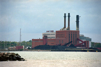
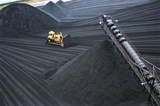
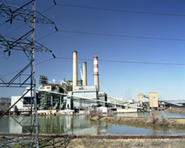
Coal
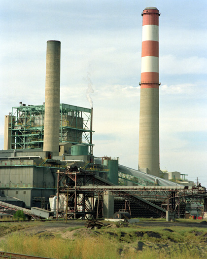
In a coal power plant:
- Heat is created: Coal is pulverized, mixed with hot air, and burned in suspension.
- Water turns to steam: The heat turns purified water into steam, which is piped to the turbine.
- Steam turns the turbine: The pressure of the steam pushes the turbine blade, turns the shaft in the generator, and creates power.
- Steam is turned back into water: Cool water is drawn into a condenser where the steam turns back into water that can be used over again in the plant.
The process outlined above is adapted from Duke Energy ("How Energy Works"). Coal plant emissions and performance are also impacted by the kind of coal (coal rank) that the plant burns. Lignite, subbituminous, bituminous, and anthracite coal are all of varying quality. The amount of moisture, sulfur, and ash in a particular type of coal can have significant influence on coal plant operation, design, and cost.
(soon to be set up for cofiring biomass)
Renewable energy technical potential, as defined by Lopez et al. (2012), represents the achievable energy generation of a particular technology given system performance, topographic limitations, and environmental and land-use constraints. Technical resource potential corresponds most closely to fossil reserves, as both can be characterized by the prospect of commercial feasibility and depend strongly on available technology at the time of the resource assessment. Coal reserves in the United States are assessed by the United States Geological Survey (USGS, "Coal Assessments").
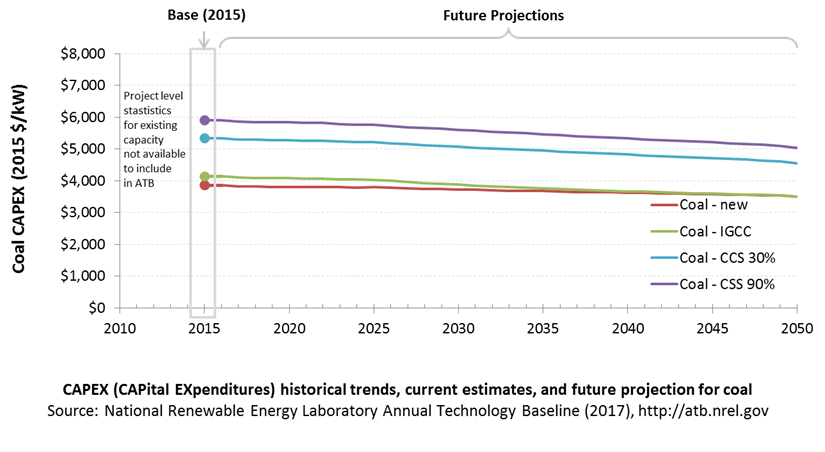
CAPital EXpenditures (CAPEX): Historical Trends, Current Estimates, and Future Projections
Technology cost and performance projections are taken the EIA Annual Energy Outlook Reference Scenario (EIA 2017). Because little-to-no coal is built in the Reference Scenario, coal capital expenditures (CAPEX) decline according to the minimum learning rate. Pulverized coal is a relatively mature technology, and therefore has a low minimum learning rate. Integrated gasification combined cycle (IGCC) technology, where the coal is gasified and then fed into a combined cycle turbine, is less mature and is assumed to have a slightly higher minimum learning rate. Coal with carbon capture and storage (CCS) is also a newer technology with a higher minimum learning rate.
Comparison with Other Sources
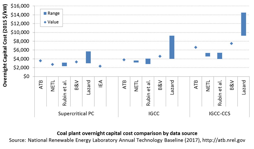
Lazard (2016) does not explicitly define their ranges with and without CCS; thus, the high end of their pulverized coal and IGCC ranges and the low end of their IGCC-CCS range are assumed to be the middle of the full reported range. All sources have been normalized to the same dollar year. Costs vary due to differences in system design (e.g., coal rank), methodology, and plant cost definitions.
CAPEX Definition
Capital expenditures (CAPEX) are expenditures required to achieve commercial operation in a given year.
For coal power plants, CAPEX equals interest during construction (ConFinFactor) times the overnight capital cost (OCC).
Overnight capital costs are modified from EIA (2017). Capital costs include overnight capital cost plus defined transmission cost, and it removes a material price index.
Fuel costs, which are just passed through to end user, are taken from EIA (2017).
For the ATB, coal-CCS technology is ultra-supercritical pulverized coal technology fitted with CCS. Both 30% capture and 90% capture options are included for the coal-CCS technology. The CCS plant configuration includes only the cost of capturing and compressing the CO2. It does not include CO2 delivery and storage.
| Overnight Capital Cost ($/kW) | Construction Financing Factor (ConFinFactor) | CAPEX ($/kW) | |
|---|---|---|---|
| Coal-new: Ultra-supercritical pulverized coal with SO2 and NOx controls | $3,559 | 1.084 | $3,859 |
| Coal-IGCC: Integrated gasification combined cycle (IGCC) | $3,819 | 1.084 | $4,141 |
| Coal-CCS: Ultra-supercritical pulverized coal with carbon capture and sequestration (CCS) options (30% / 90% capture) | $4,927 / $5,448 | 1.084 | $5,341 / $5,906 |
CAPEX can be determined for a plant in a specific geographic location as follows:
CAPEX = ConFinFactor × (OCC×CapRegMult+GCC).
(See the Financial Definitions tab in the ATB data spreadsheet.)
Regional cost variations and geographically specific grid connection costs are not included in the ATB (CapRegMult=1; GCC=0). In the ATB, the input value is overnight capital cost (OCC) and details to calculate interest during construction (ConFinFactor).
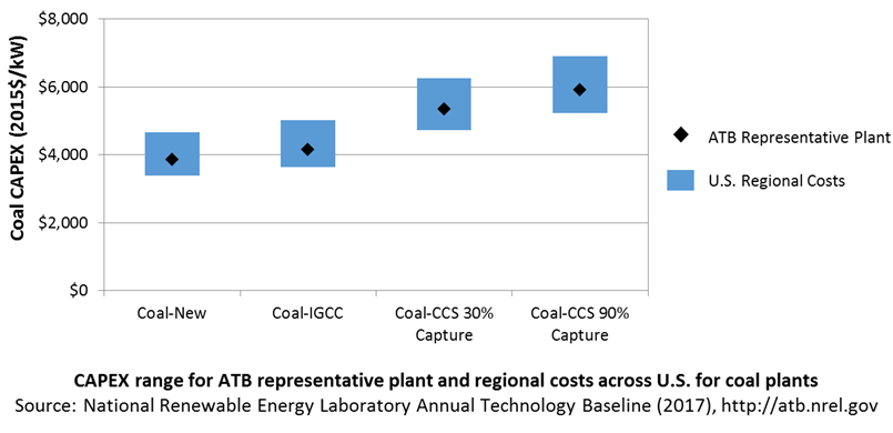
In the ATB, CAPEX represents each type of a coal plant with a unique value. Regional cost effects associated with labor rates, material costs, and other regional effects as defined by EIA (2016a) expand the range of CAPEX. Unique land-based spur line costs based on distance and transmission line costs are not estimated. The following figure illustrates the ATB representative plant relative to the range of CAPEX including regional costs across the contiguous United States. The ATB representative plants are associated with a regional multiplier of 1.0.
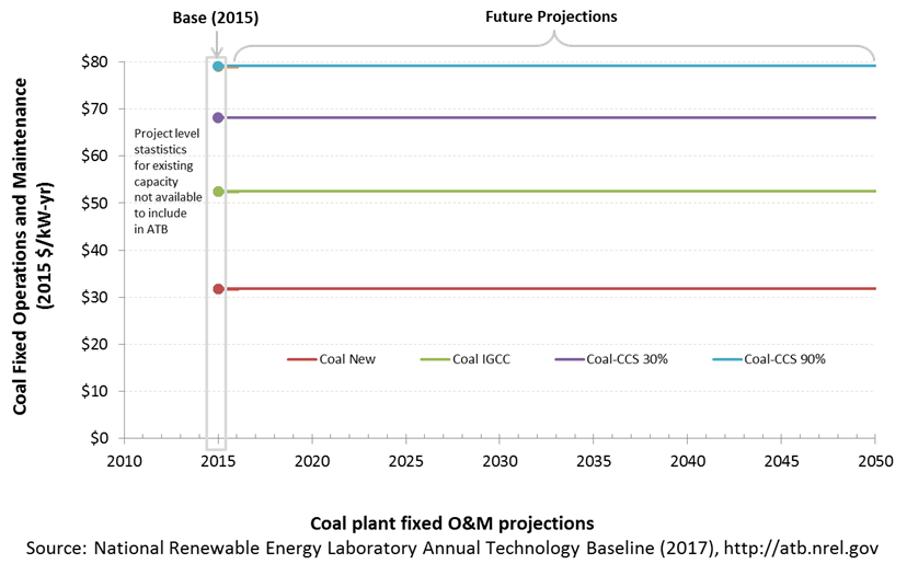
Operation and Maintenance (O&M) Costs
Operations and maintenance (O&M) costs represent the annual expenditures required to operate and maintain a plant over its technical lifetime (the distinction between economic life and technical life is described here), including:
- Insurance, taxes, land lease payments, and other fixed costs
- Present value and annualized large component replacement costs over technical life
- Scheduled and unscheduled maintenance of power plants, transformers, and other components over the technical lifetime of the plant.
Market data for comparison are limited and generally inconsistent in the range of costs covered and the length of the historical record.
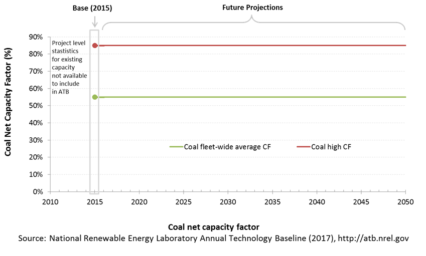
Capacity Factor: Expected Annual Average Energy Production Over Lifetime
The capacity factor represents the assumed annual energy production divided by the total possible annual energy production, assuming the plant operates at rated capacity for every hour of the year. For coal plants, the capacity factors are typically lower than their availability factors. Coal plant availability factors have a wide range depending on system design and maintenance schedules.
The capacity factor of dispatchable units is typically a function of the unit's marginal costs and local grid needs (e.g., need for voltage support or limits due to transmission congestion).
Coal power plants have typically been operated as baseload units, although that has changed in many locations due to low natural gas prices and increased penetration of variable renewable technologies. The average capacity factor used in the ATB is the fleet-wide average reported by EIA for 2015. The high capacity factor represents a new plant that would operate as a baseload unit.
Even though IGCC and coal with CCS have experienced limited deployment in the United States, it is expected that their performance characteristics would be similar to new coal power plants.
Levelized Cost of Energy (LCOE) Projections
Levelized cost of energy (LCOE) is a simple metric that combines the primary technology cost and performance parameters, CAPEX, O&M, and capacity factor. It is included in the ATB for illustrative purposes. The focus of the ATB is to define the primary cost and performance parameters for use in electric sector modeling or other analysis where more sophisticated comparisons among technologies are made. LCOE captures the energy component of electric system planning and operation, but the electric system also requires capacity and flexibility services to operate reliably. Electricity generation technologies have different capabilities to provide such services. For example, wind and PV are primarily energy service providers, while the other electricity generation technologies provide capacity and flexibility services in addition to energy. These capacity and flexibility services are difficult to value and depend strongly on the system in which a new generation plant is introduced. These services are represented in electric sector models such as the ReEDS model and corresponding analysis results such as the Standard Scenarios.
The following three figures illustrate the combined impact of CAPEX, O&M, and capacity factor projections across the range of resources present in the contiguous United States. The Current Market Conditions LCOE demonstrates the range of LCOE based on macroeconomic conditions similar to the present. The Historical Market Conditions LCOE presents the range of LCOE based on macroeconomic conditions consistent with prior ATB editions and Standard Scenarios model results. The Normalized LCOE (all LCOE estimates are normalized with the lowest Base Year LCOE value) emphasizes the relative effect of fuel price and heat rate independent of project finance assumptions. The ATB representative plant characteristics that best align with recently installed or anticipated near-term coal plants are associated with Coal-New-HighCF. Data for all the resource categories can be found in the ATB data spreadsheet.
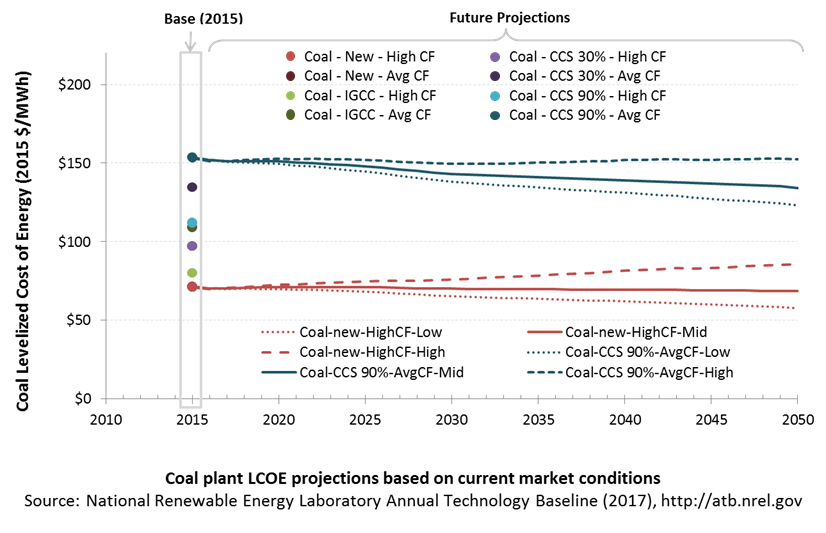
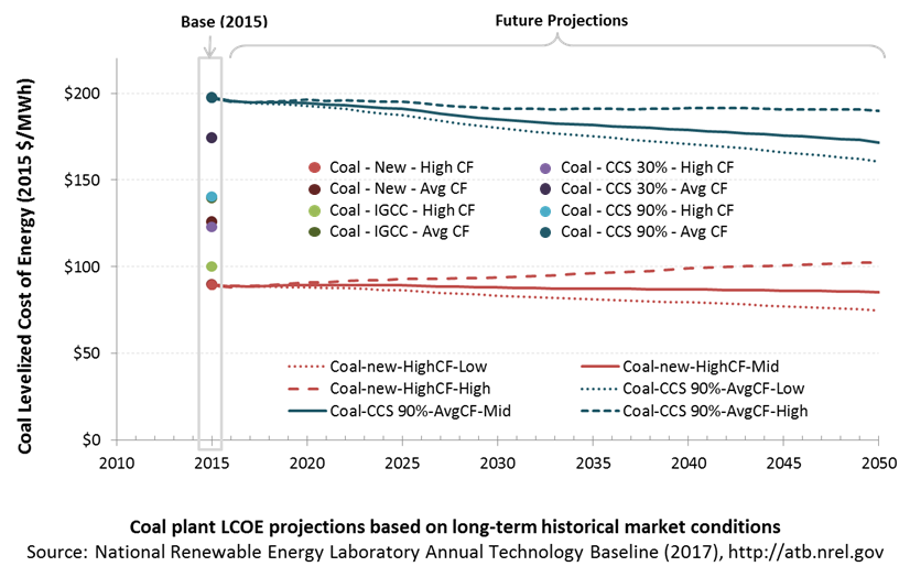
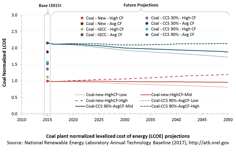
The LCOE of coal power plants is directly impacted by multiple coal fuel cost scenarios. It is also impacted by variations in the heat rate, O&M costs, and assumed capacity factor. For a given year, the LCOE assumes that the fuel prices from that year continue throughout the lifetime of the plant.
The projections do not include any cost of carbon, which would influence the LCOE of fossil units. Also, for CCS plants, the potential revenue from selling the captured carbon is not included (e.g., enhanced oil recovery operation may purchase CO2 from a CCS plant).
To estimate LCOE, assumptions about the cost of capital to finance electricity generation projects are required. For comparison in the ATB, two project finance structures are represented.
- Current Market Conditions: The values of the production tax credit (PTC) and investment tax credit (ITC) are ramping down by 2020, at which time wind and solar projects may be financed with debt fractions similar to other technologies. This scenario reflects debt interest (4.4% nominal, 1.9% real) and return on equity rates (9.5% nominal, 6.8% real) to represent 2017 market conditions (AEO 2017) and a debt fraction of 60% for all electricity generation technologies. An economic life, or period over which the initial capital investment is recovered, of 20 years is assumed for all technologies. These assumptions are one of the project finance options in the ATB spreadsheet.
- Long-Term Historical Market Conditions: Historically, debt interest and return on equity were represented with higher values. This scenario reflects debt interest (8% nominal, 5.4% real) and return on equity rates (13% nominal, 10.2% real) implemented in the ReEDS model and reflected in prior versions of the ATB and Standard Scenarios model results. A debt fraction of 60% for all electricity generation technologies is assumed. An economic life, or period over which the initial capital investment is recovered, of 20 years is assumed for all technologies. These assumptions are one of the project finance options in the ATB spreadsheet.
These parameters are held constant for estimates representing the Base Year through 2050. No incentives such as the PTC or ITC are included. The equations and variables used to estimate LCOE are defined on the equations and variables page. For illustration of the impact of changing financial structures such as WACC and economic life, see Project Finance Impact on LCOE. For LCOE estimates for High, Mid, and Low scenarios for all technologies, see 2017 ATB Cost and Performance Summary.
Biopower Plants
In a biopower plant:
- Heat is created: Biomass (sometimes co-fired with coal) is pulverized, mixed with hot air, and burned in suspension.
- Water turns to steam: The heat turns purified water into steam, which is piped to the turbine.
- Steam turns the turbine: The pressure of the steam pushes the turbine blade, turns the shaft in the generator, and creates power.
- Steam is turned back into water: Cool water is drawn into a condenser where the steam turns back into water that can be reused in the plant.
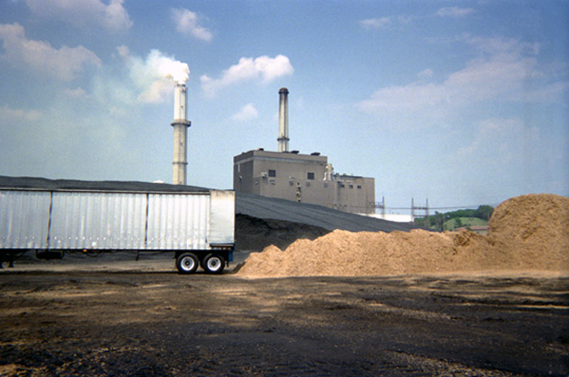
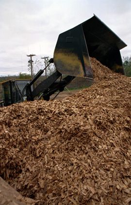
(a biomass gasifier that operates on wood chips)
Renewable energy technical potential, as defined by Lopez et al. (2012), represents the achievable energy generation of a particular technology given system performance, topographic limitations, and environmental and land-use constraints. Technical resource potential for biopower is based on estimated biomass quantities from the Billion Ton Update study (DOE 2011).
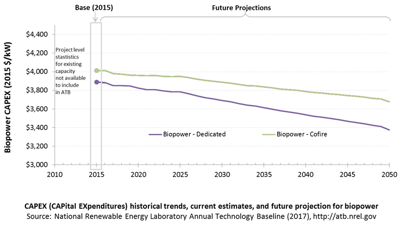
CAPital EXpenditures (CAPEX): Historical Trends, Current Estimates, and Future Projections
Because biopower plants are well-known and perform close to their optimal performance, EIA expects capital expenditures (CAPEX) will incrementally improve over time and slightly more quickly than inflation.
The exception is new biomass cofiring, which is expected to have costs that decline a bit more than existing cofiring project technologies.
CAPEX Definition
Capital expenditures (CAPEX) are expenditures required to achieve commercial operation in a given year.
Overnight capital costs are modified from EIA (2014). Capital costs include overnight capital cost plus defined transmission cost, and it removes a material price index. The overnight capital costs for cofired units are not the cost of upgrading a plant but the total cost of the plant after the upgrade.
Fuel costs are taken from the Billion Ton Update study (DOE 2011).
| Overnight Capital Cost ($/kW) | Construction Financing Factor (ConFinFactor) | CAPEX ($/kW) | |
|---|---|---|---|
| Dedicated: Dedicated biopower plant | $3,737 | 1.041 | $3,889 |
| CofireOld: Pulverized coal with sulfur dioxide (SO2) scrubbers and biomass co-firing | $3,856 | 1.041 | $4,013 |
| CofireNew: Advanced supercritical coal with SO2 and NOx controls and biomass co-firing | $3,856 | 1.041 | $4,013 |
CAPEX can be determined for a plant in a specific geographic location as follows:
CAPEX = ConFinFactor*(OCC*CapRegMult+GCC).
(See the Financial Definitions tab in the ATB data spreadsheet.)
Regional cost variations and geographically specific grid connection costs are not included in the ATB (CapRegMult = 1; GCC = 0). In the ATB, the input value is overnight capital cost (OCC) and details to calculate interest during construction (ConFinFactor).
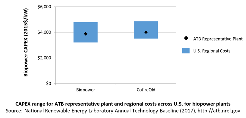
In the ATB, CAPEX represents each type of biopower plant with a unique value. Regional cost effects associated with labor rates, material costs, and other regional effects as defined by EIA (2016a) expand the range of CAPEX. Unique land-based spur line costs based on distance and transmission line costs are not estimated. The following figure illustrates the ATB representative plant relative to the range of CAPEX including regional costs across the contiguous United States. The ATB representative plants are associated with a regional multiplier of 1.0.
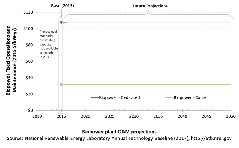
Operation and Maintenance (O&M) Costs
Operations and maintenance (O&M) costs represent the annual expenditures required to operate and maintain a plant over its technical lifetime (the distinction between economic life and technical life is described here), including:
- Insurance, taxes, land lease payments, and other fixed costs
- Present value and annualized large component replacement costs over technical life
- Scheduled and unscheduled maintenance of power plants, transformers, and other components over the technical lifetime of the plant.
Market data for comparison are limited and generally inconsistent in the range of costs covered and the length of the historical record.
Capacity Factor: Expected Annual Average Energy Production Over Lifetime
The capacity factor represents the assumed annual energy production divided by the total possible annual energy production, assuming the plant operates at rated capacity for every hour of the year. For biopower plants, the capacity factors are typically lower than their availability factors. Biopower plant availability factors have a wide range depending on system design, fuel type and availability, and maintenance schedules.
Biopower plants are typically baseload plants with steady capacity factors. For the ATB, the biopower capacity factor is taken as the average capacity factor for biomass plants for 2015, as reported by EIA.
Biopower capacity factors are influenced by technology and feedstock supply, expected downtime, and energy losses.

Levelized Cost of Energy (LCOE) Projections
Levelized cost of energy (LCOE) is a simple metric that combines the primary technology cost and performance parameters, CAPEX, O&M, and capacity factor. It is included in the ATB for illustrative purposes. The focus of the ATB is to define the primary cost and performance parameters for use in electric sector modeling or other analysis where more sophisticated comparisons among technologies are made. LCOE captures the energy component of electric system planning and operation, but the electric system also requires capacity and flexibility services to operate reliably. Electricity generation technologies have different capabilities to provide such services. For example, wind and PV are primarily energy service providers, while the other electricity generation technologies provide capacity and flexibility services in addition to energy. These capacity and flexibility services are difficult to value and depend strongly on the system in which a new generation plant is introduced. These services are represented in electric sector models such as the ReEDS model and corresponding analysis results such as the Standard Scenarios.
The following three figures illustrate the combined impact of CAPEX, O&M, and capacity factor projections across the range of resources present in the contiguous United States. The Current Market Conditions LCOE demonstrates the range of LCOE based on macroeconomic conditions similar to the present. The Historical Market Conditions LCOE presents the range of LCOE based on macroeconomic conditions consistent with prior ATB editions and Standard Scenarios model results. The Normalized LCOE (all LCOE estimates are normalized with the lowest Base Year LCOE value) emphasizes the relative effect of fuel price and heat rate independent of project finance assumptions. Data for all the resource categories can be found in the ATB data spreadsheet.
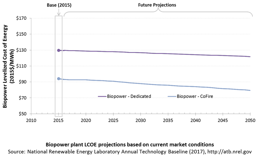
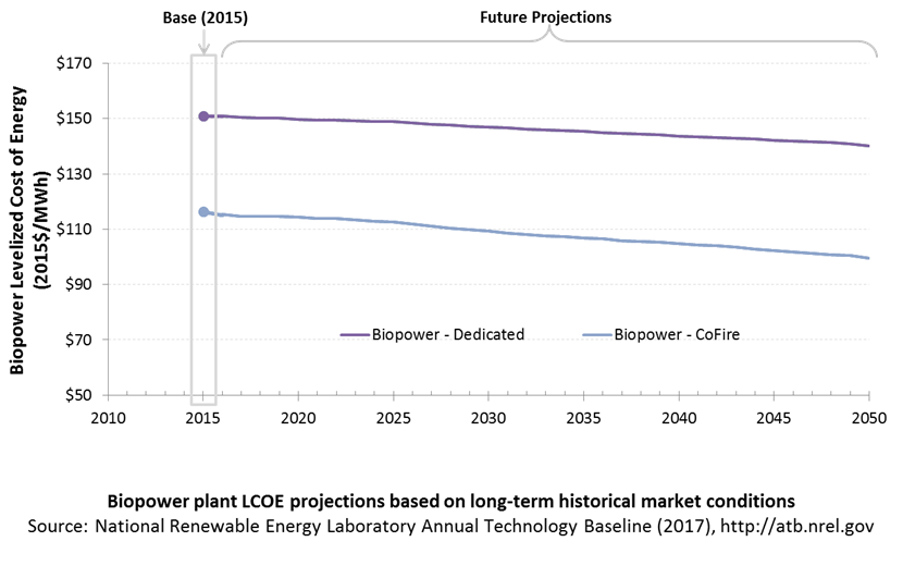
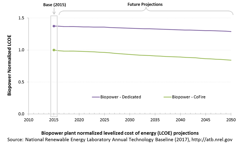
The LCOE of biopower plants is directly impacted by the differences in CAPEX (installed capacity costs) as well as by heat rate differences. For a given year, the LCOE assumes that the fuel prices from that year continue throughout the lifetime of the plant.
Regional variations will ultimately impact biomass feedstock costs, but these are not included in the ATB.
The projections do not include any cost of carbon.
Fuel prices are based on the EIA's Annual Energy Outlook 2017 (EIA 2017).
To estimate LCOE, assumptions about the cost of capital to finance electricity generation projects are required. For comparison in the ATB, two project finance structures are represented.
- Current Market Conditions: The values of the production tax credit (PTC) and investment tax credit (ITC) are ramping down by 2020, at which time wind and solar projects may be financed with debt fractions similar to other technologies. This scenario reflects debt interest (4.4% nominal, 1.9% real) and return on equity rates (9.5% nominal, 6.8% real) to represent 2017 market conditions (AEO 2017) and a debt fraction of 60% for all electricity generation technologies. An economic life, or period over which the initial capital investment is recovered, of 20 years is assumed for all technologies. These assumptions are one of the project finance options in the ATB spreadsheet.
- Long-Term Historical Market Conditions: Historically, debt interest and return on equity were represented with higher values. This scenario reflects debt interest (8% nominal, 5.4% real) and return on equity rates (13% nominal, 10.2% real) implemented in the ReEDS model and reflected in prior versions of the ATB and Standard Scenarios model results. A debt fraction of 60% for all electricity generation technologies is assumed. An economic life, or period over which the initial capital investment is recovered, of 20 years is assumed for all technologies. These assumptions are one of the project finance options in the ATB spreadsheet.
These parameters are held constant for estimates representing the Base Year through 2050. No incentives such as the PTC or ITC are included. The equations and variables used to estimate LCOE are defined on the equations and variables page. For illustration of the impact of changing financial structures such as WACC and economic life, see Project Finance Impact on LCOE. For LCOE estimates for High, Mid, and Low scenarios for all technologies, see 2017 ATB Cost and Performance Summary.
References
Augustine, C. 2011. Updated U.S. Geothermal Supply Characterization and Representation for Market Penetration Input. Golden, CO: National Renewable Energy Laboratory. NREL/TP-6A2-47459. October 2011. http://www.nrel.gov/docs/fy12osti/47459.pdf.
B&V (Black & Veatch). 2012. Cost and Performance Data for Power Generation Technologies. Black & Veatch Corporation. February 2012. http://bv.com/docs/reports-studies/nrel-cost-report.pdf.
DOE (U.S. Department of Energy). 2011. U.S. Billion-Ton Update: Biomass Supply for a Bioenergy and Bioproducts Industry. Perlack, R.D., and B.J. Stokes, eds. Oak Ridge, TN: Oak Ridge National Laboratory. ORNL/TM-2011/224. August 2011. https://www.osti.gov/scitech/biblio/1023318.
EIA (U.S. Energy Information Administration). 2014. Annual Energy Outlook 2014 with Projections to 2040. Washington, D.C.: U.S. Department of Energy. DOE/EIA-0383(2014). April 2014. http://www.eia.gov/forecasts/aeo/pdf/0383(2014).pdf.
EIA (U.S. Energy Information Administration). 2015. Annual Energy Outlook with Projections to 2040. Washington, D.C.: U.S. Department of Energy. DOE/EIA-0383(2015). April 2015. http://www.eia.gov/outlooks/aeo/pdf/0383(2015).pdf.
EIA (U.S. Energy Information Administration). 2016a. Capital Cost Estimates for Utility Scale Electricity Generating Plants. Washington, D.C.: U.S. Department of Energy. November 2016. https://www.eia.gov/analysis/studies/powerplants/capitalcost/pdf/capcost_assumption.pdf.
EIA (U.S. Energy Information Administration). 2017. Annual Energy Outlook 2017 with Projections to 2050. Washington, D.C.: U.S. Department of Energy. January 5, 2017. http://www.eia.gov/outlooks/aeo/pdf/0383(2017).pdf.
IEA (International Energy Agency). 2017. Reference to come.
Lazard. 2016. Levelized Cost of Energy Analysis-Version 10.0. December 2016. New York: Lazard. https://www.lazard.com/media/438038/levelized-cost-of-energy-v100.pdf.
Lopez, Anthony, Billy Roberts, Donna Heimiller, Nate Blair, and Gian Porro. 2012. U.S. Renewable Energy Technical Potentials: A GIS-Based Analysis. National Renewable Energy Laboratory. NREL/TP-6A20-51946. http://www.nrel.gov/docs/fy12osti/51946.pdf.
Mines, Greg. 2013. Geothermal Electricity Technology Evaluation Model. Geothermal Technologies Office. 2013 Peer Review. Washington, D.C: U.S. Department of Energy. April 22, 2013. https://energy.gov/sites/prod/files/2014/02/f7/mines_getem_peer2013.pdf.
MIT (Massachusetts Institute of Technology), and INL (Idaho National Laboratory). 2006. The Future of Geothermal Energy Impact of Enhanced Geothermal Systems (EGS) on the United States in the 21st Century. Idaho Falls, ID: Idaho National Laboratory. INL/EXT-06-11746. November 2006. https://energy.mit.edu/wp-content/uploads/2006/11/MITEI-The-Future-of-Geothermal-Energy.pdf.
NETL (National Energy Technology Laboratory: Tim Fout, Alexander Zoelle, Dale Keairns, Marc Turner, Mark Woods, Norma Kuehn, Vasant Shah, Vincent Chou, Lora Pinkerton). 2015. Fossil Energy Plants: Volume 1a: Bituminous Coal (PC) and Natural Gas to Electricity, Revision 3. DOE/NETL-2015/1723. http://www.netl.doe.gov/File%20Library/Research/Energy%20Analysis/Publications/Rev3Vol1aPC_NGCC_final.pdf.
Rubin, Edward S., Inês M.L. Azevedo, Paulina Jaramillo, and Sonia Yeh. 2015. 'A Review of Learning Rates for Electricity Supply Technologies.' Energy Policy 86 (November 2015): 198–218. http://www.sciencedirect.com/science/article/pii/S0301421515002293.
Williams, Colin F., Marshall J. Reed, Robert H. Mariner, Jacob DeAngelo, S. Peter Galanis, Jr. 2008. 'Assessment of Moderate- and High-Temperature Geothermal Resources of the United States.' Menlo Park, CA: U.S. Geological Survey. Fact Sheet 2008-3082. September 2008. https://pubs.usgs.gov/fs/2008/3082/.