Annual Technology Baseline 2017
National Renewable Energy Laboratory
Recommended Citation:
NREL (National Renewable Energy Laboratory). 2017. 2017 Annual Technology Baseline. Golden, CO: National Renewable Energy Laboratory. http://atb.nrel.gov/.
Please consult Guidelines for Using ATB Data:
https://atb.nrel.gov/electricity/user-guidance.html
Land-Based Wind Power Plants
Representative Technology
Most land-based wind plants in the United States range in capacity from 50 MW to 100 MW (Wiser and Bolinger 2015). Wind turbines installed in the United States in 2015 were, on average, 2-MW turbines with rotor diameters of 102 m and hub heights of 82 m (Moné et al. 2017).
Resource Potential
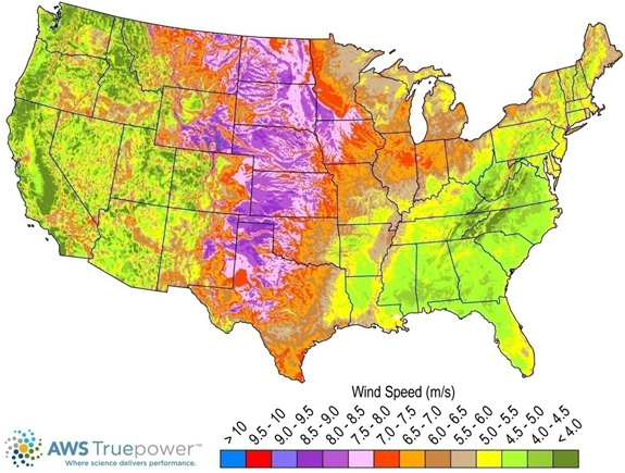
Wind resource is prevalent throughout the United States but is concentrated in the central states. Total land-based wind technical potential exceeds 10,000 GW (almost tenfold current total U.S. electricity generation capacity), which corresponds to over 3.5 million km2 of potential land area after accounting for standard exclusions such as federally protected areas, urban areas, and water. Resource potential has been expanded from approximately 6,000 GW (DOE 2015) by including locations with lower wind speeds to provide more comprehensive coverage of U.S. land areas where future technology may improve economic potential.
Renewable energy technical potential, as defined by Lopez et al. (2012), represents the achievable energy generation of a particular technology given system performance, topographic limitations and environmental and land-use constraints. The primary benefit of assessing technical potential is that it establishes an upper-boundary estimate of development potential. It is important to understand that there are multiple types of potential-resource, technical, economic, and market (Lopez et al. 2012; NREL, "Renewable Energy Technical Potential").
The resource potential is calculated by using over 130,000 distinct areas for wind plant deployment that cover over 3.5 million km2. The potential capacity is estimated to total over 10,000 GW if a packing density of 3MW/km2 is assumed.
Base Year and Future Year Projections Overview
For each of the 130,000 distinct areas, an LCOE is estimated taking into consideration site-specific hourly wind profiles. Five different wind turbines are associated with a range of average annual wind speed based on actual wind plant installations in 2015. This method is described in Moné et al, (2017) and summarized below.
- The capital expenditures (CAPEX) associated with wind plants installed in 2015 in the interior of the country are used to represent wind plants associated with average annual wind speeds that correspond with the median wind speed for projects installed in 2015. A range of CAPEX across the range of wind speeds is developed using engineering models and assumed differences in rotor diameter. Wind turbines at lower wind speed sites have larger rotors and, therefore, higher CAPEX.
- The capacity factor is determined for each unique geographic location using the site-specific hourly wind profile and a power curve that corresponds with the five wind turbines defined to represent the range of wind technology installed in the United States in 2015.
- Average annual operations and maintenance (O&M) costs are assumed equivalent at all geographic locations.
- LCOE is calculated for each area based on the CAPEX and capacity factor estimated for each area.
For illustration in the ATB, the full resource potential, represented by 130,000 areas, was divided into 10 techno-resource groups (TRGs). The capacity-weighted average CAPEX, O&M, and capacity factor for each group is presented in the ATB.
Future year projections are derived from estimated cost reduction potential for land-based wind technologies based on elicitation of over 160 wind industry experts (Wiser et al. 2016). This study produced three different cost reduction pathways, and the median and low estimates for LCOE reduction are used for ATB Mid and ATB Low cost scenarios. Because the overall LCOE reduction was used as the basis for the ATB projections, all three cost elements - CAPEX, O&M, and capacity factor - should be considered together. The individual component projections are illustrative. Three different projections were developed for scenario modeling as bounding levels:
- High cost: no change in CAPEX, O&M, or capacity factor from 2015 to 2050; consistent across all renewable energy technologies in the ATB
- Mid cost: LCOE percent reduction from the Base Year equivalent to that corresponding to the Median Scenario (50% probability) in expert survey (Wiser et al. 2016)
- Low Cost: LCOE percent reduction from the Base Year equivalent to that corresponding to the Low Scenario (10% probability) in expert survey (Wiser et al. 2016).
CAPital EXpenditures (CAPEX): Historical Trends, Current Estimates, and Future Projections
Capital expenditures (CAPEX) are expenditures required to achieve commercial operation in a given year. These expenditures include the wind turbine, the balance of system (e.g., site preparation, installation, and electrical infrastructure), and financial costs (e.g., development costs, onsite electrical equipment, and interest during construction) and are detailed in CAPEX Definition. In the ATB, CAPEX reflects typical plants and does not include differences in regional costs associated with labor or materials. The range of CAPEX demonstrates variation with wind resource in the contiguous United States.
The following figure shows the Base Year estimate and future year projections for CAPEX costs. Three cost reduction scenarios are represented: High, Mid, and Low. Historical data from land-based wind plants installed in the United States are shown for comparison to the ATB Base Year estimates. The estimate for a given year represents CAPEX of a new plant that reaches commercial operation in that year.
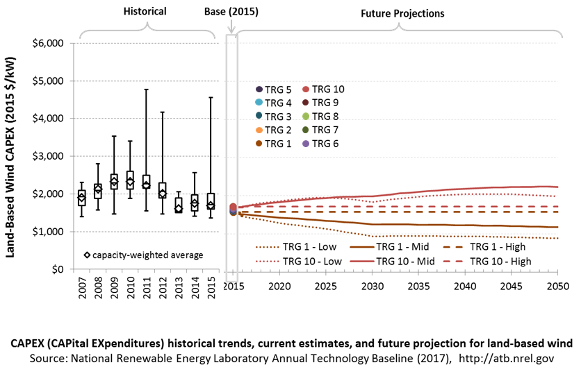
CAPEX estimates for 2015 correspond well with market data for plants installed in 2015. Projections reflect a continuation of the downward trend observed in the recent past and are anticipated to continue based on preliminary data for 2016 projects.
In the lower wind resource areas represented by TRGs 6-10, CAPEX is likely to grow as future wind turbine technology transitions to new platforms, including taller towers, larger rotors, and higher machine ratings. In the higher wind resource areas represented by TRGs 1-5, optimization of current wind turbine platforms will lead to lower CAPEX in future years.
Recent Trends
Actual land-based wind plant CAPEX (Wiser et al. 2014) is shown in box-and-whiskers format for comparison to the ATB current CAPEX estimates and future projections. Wiser and Bolinger (2014) provide statistical representation of CAPEX for about 65% of wind plants installed in the United States since 2007.
CAPEX estimates should tend toward the low end of observed cost because no regional impacts or spur line costs are included. These effects are represented in the market data.
Base Year Estimates
For illustration in the ATB, all potential land-based wind plant areas were represented in 10 TRGs. These were defined by resource potential (GW) and with higher resolution on the highest-quality TRGs, as these are the most likely sites to be deployed, based on their economics.
TRG 1 represents the best 100 GW of wind, as determined by LCOE. TRG 2 represents the next best 200 GW, while TRG 3 represents the next best 400 GW, and TRG 4 represents the next best 800 GW. TRGs 5-9 all represent 1,600 GW of resource potential. TRG 10 represents the remaining 1,148 GW of available potential. This representation is based on the approach described in DOE (2015) and implemented with 2015 market data in Moné et al. (2017).
The table below summarizes the annual average wind speed range for each TRG, capacity-weighted average wind speed, cost and performance parameters for each TRG, and resource potential in terms of capacity and energy for each TRG. Typical land-based wind installations in 2015 are associated with TRG 4.
| Techno-Resource Group (TRG) | Wind Speed Range (m/s) | Weighted Average Wind Speed (m/s) | Weighted Average CAPEX ($/kW) | Weighted Average OPEX ($/kW/yr) | Weighted Average Net CF (%) | Potential Wind Plant Capacity (GW) | Potential Wind Plant Energy (TWh) |
|---|---|---|---|---|---|---|---|
| TRG1 | 8.2–13.5 | 8.7 | 1,573 | 51 | 47.4% | 100 | 414 |
| TRG2 | 8.0–10.9 | 8.4 | 1,592 | 51 | 46.2% | 200 | 810 |
| TRG3 | 7.7–11.1 | 8.2 | 1,599 | 51 | 45.0% | 400 | 1,576 |
| TRG4 | 7.5–13.1 | 7.9 | 1,605 | 51 | 43.5% | 800 | 3,050 |
| TRG5 | 6.9–11.1 | 7.5 | 1,616 | 51 | 40.7% | 1,600 | 5,708 |
| TRG6 | 6.1–9.4 | 6.9 | 1,642 | 51 | 36.4% | 1,600 | 5,098 |
| TRG7 | 5.4–8.3 | 6.2 | 1,678 | 51 | 30.8% | 1,600 | 4,320 |
| TRG8 | 4.7–6.9 | 5.5 | 1,708 | 51 | 24.6% | 1,600 | 3,443 |
| TRG9 | 4.0–6.0 | 4.8 | 1,713 | 51 | 18.3% | 1,600 | 2,558 |
| TRG10 | 1.0–5.3 | 4.0 | 1,713 | 51 | 11.1% | 1,148 | 1,116 |
| Total | 10,648 | 28,092 | |||||
Future Year Projections
Projections of future LCOE were derived from a survey of wind industry experts (Wiser et al. 2016) for scenarios that are associated with 50% and 10% probability levels in 2030 and 2050. Projections of future offshore wind plant CAPEX was determined based on adjustments to CAPEX, fixed O&M (FOM), and capacity factor in each year to result in a predetermined LCOE value based on an expert survey conducted by Wiser et al. (2016).
In order to achieve the overall LCOE reduction associated with the median and low projections from the expert survey, CAPEX was used to accommodate all improvement aspects other than O&M and capacity factor survey results. In the lower wind resource areas represented by TRGs 6-10, CAPEX is likely to grow as future wind turbine technology transitions to new platforms, including taller towers, larger rotors, and higher machine ratings. In the higher wind resource areas represented by TRGs 1-5, optimization of current wind turbine platforms will lead to lower CAPEX.
A detailed description of the methodology for developing future year projections is found in Projections Methodology.
Technology innovations that could impact future CAPEX costs are summarized in LCOE Projections.
CAPEX Definition
Capital expenditures (CAPEX) are expenditures required to achieve commercial operation in a given year.
For the ATB - and based on EIA (2016a) and the System Cost Breakdown Structure defined by Moné et al. (2015) - the wind plant envelope is defined to include:
- Wind turbine supply
- Balance of system (BOS)
- Turbine installation, substructure supply, and installation
- Site preparation, installation of underground utilities, access roads, and buildings for operations and maintenance
- Electrical infrastructure, such as transformers, switchgear, and electrical system connecting turbines to each other and to the control center
- Project-related indirect costs, including engineering, distributable labor and materials, construction management start up and commissioning, and contractor overhead costs, fees, and profit.
- Financial costs
- Owner's costs, such as development costs, preliminary feasibility and engineering studies, environmental studies and permitting, legal fees, insurance costs, and property taxes during construction
- Onsite electrical equipment (e.g., switchyard), a nominal-distance spur line (^lt;1 mile), and necessary upgrades at a transmission substation; distance-based spur line cost (GCC) not included in the ATB
- Interest during construction estimated based on three-year duration accumulated 10%/10%/80% at half-year intervals and an 8% interest rate (ConFinFactor).
CAPEX can be determined for a plant in a specific geographic location as follows:
CAPEX = ConFinFactor*(OCC*CapRegMult+GCC).
(See the Financial Definitions tab in the ATB data spreadsheet.)
Regional cost variations and geographically specific grid connection costs are not included in the ATB (CapRegMult = 1; GCC = 0). In the ATB, the input value is overnight capital cost (OCC) and details to calculate interest during construction (ConFinFactor).
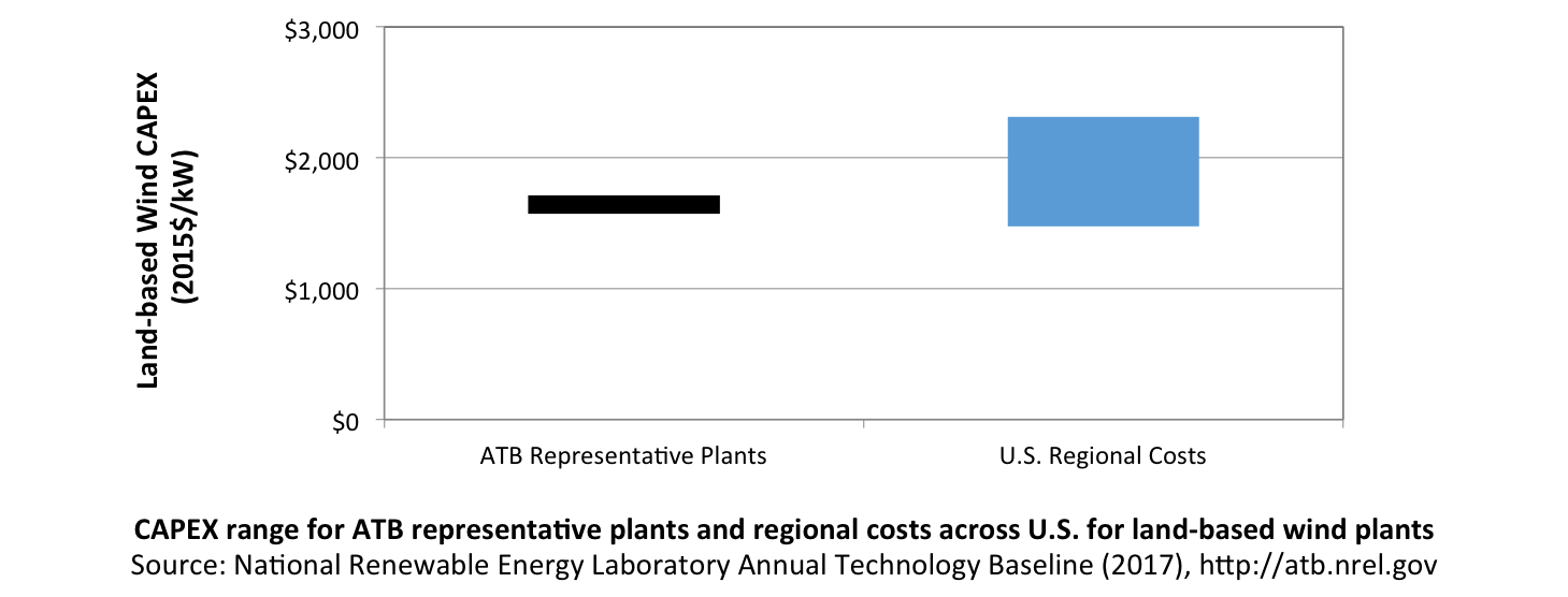
In the ATB, CAPEX represents a typical land-based wind plant and varies with annual average wind speed. Regional cost effects associated with labor rates, material costs, and other regional effects as defined by EIA (2016a), DOE (2015) expand the range of CAPEX. Unique land-based spur line costs for each of the 130,000 areas based on distance and transmission line costs expand the range of CAPEX even further. The figure below illustrates the ATB representative plants relative to the range of CAPEX including regional costs across the contiguous United States. Note that the ATB Base Year estimate for TRG 4 is equivalent to the market data observed capacity-weighted average wind plant CAPEX in the same year. The ATB representative plants are associated with a regional multiplier of 1.0.
Standard Scenarios Model Results
ATB CAPEX, O&M, and capacity factor assumptions for Base Year and future projections through 2050 for High, Mid, and Low projections are used to develop the NREL Standard Scenarios using the ReEDS model. See ATB and ATB and Standard Scenarios.
CAPEX in the ATB does not represent regional variants (CapRegMult) associated with labor rates, material costs, etc., but the ReEDS model does include 134 regional multipliers (EIA 2016a).
The ReEDS model determines the land-based spur line (GCC) uniquely for each of the 130,000 areas based on distance and transmission line cost.
Operation and Maintenance (O&M) Costs
Operations and maintenance (O&M) costs represent the annual fixed expenditures (and depend on capacity) required to operate and maintain a wind plant over its technical lifetime of 25 years (the distinction between economic life and technical life is described here), including:
- Insurance, taxes, land lease payments, and other fixed costs
- Present value, annualized large component costs over technical life (e.g., blades, gearboxes, generators)
- Scheduled and unscheduled maintenance of wind plant components including turbines, transformers, etc. over the technical lifetime of the plant.
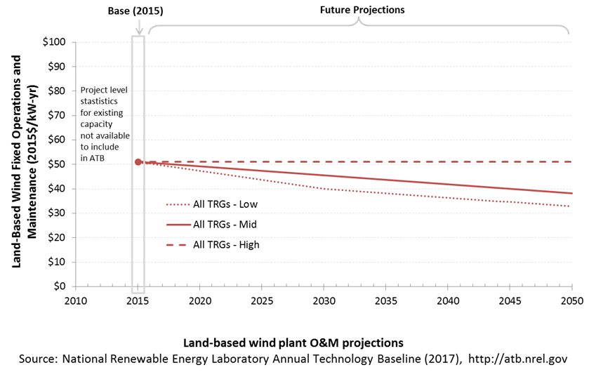
The following figure shows the Base Year estimate and future year projections for fixed O&M (FOM) costs. Three cost reduction scenarios are represented. The estimate for a given year represents annual average FOM costs expected over the technical lifetime of a new plant that reaches commercial operation in that year.
Base Year Estimates
Due to a lack of robust market data, an assumption of FOM of $51/kW-yr was determined to be representative of the range of available data; no variation of FOM with TRG (or wind speed) was assumed (DOE 2015).
Future Year Projections
Future FOM is assumed to decline 25% by 2050 in Mid cost case and 39% in Low cost wind cases. These values are the result of linear curves fit to the results of the expert survey documented in Wiser et al. (2016).
A detailed description of the methodology for developing future year projections is found in Projections Methodology. A detailed description of the methodology for developing future year projections is found in Projections Methodology.
Technology innovations that could impact future O&M costs are summarized in LCOE Projections.
Capacity Factor: Expected Annual Average Energy Production Over Lifetime
The capacity factor represents the expected annual average energy production divided by the annual energy production, assuming the plant operates at rated capacity for every hour of the year. It is intended to represent a long-term average over the technical lifetime of the plant (the distinction between economic life and technical life is described here). It does not represent interannual variation in energy production. Future year estimates represent the estimated annual average capacity factor over the technical lifetime of a new plant installed in a given year.
The capacity factor is influenced by hourly wind profile, expected downtime, and energy losses within the wind plant. The specific power (ratio of machine rating to rotor swept area) and hub height are design choices that influence the capacity factor.
The following figure shows a range of capacity factors based on variation in the resource for wind plants in the contiguous United States. Historical data from wind plants operating in the United States in 2015, according to the year in which plants were installed, is shown for comparison to the ATB Base Year estimates. The range of Base Year estimates illustrate the effect of locating a wind plant in sites with high wind speeds (TRG 1) or low wind speeds (TRG 10). Future projections are shown for High, Mid, and Low cost scenarios.
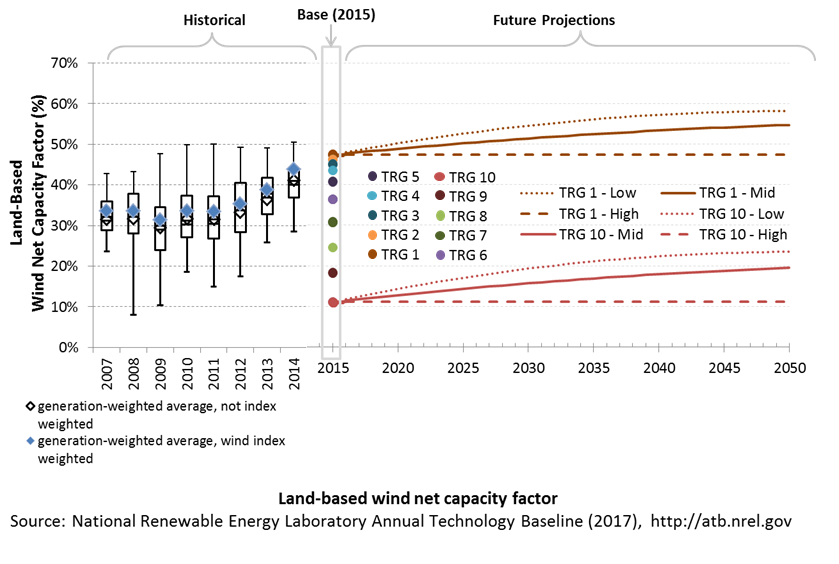
Recent Trends
Actual energy production from about 90% of wind plants operating in the United States since 2007 (Wiser et al. 2014) is shown in box-and-whiskers format for comparison with the ATB current estimates and future projections. The historical data illustrate capacity factor for projects operating in 2015, shown by year of commercial online date. As reported in the 2015 DOE Wind Technologies Market Report (Wiser and Bolinger 2016), NextEra Energy Resources, in their quarterly earnings reports, estimates that the "wind resource index" for the United States as a whole was 94% in 2015. The generation-weighted average 2015 capacity factors are also shown adjusted upward for a typical wind resource year by 1/0.94.
Base Year Estimates
For illustration in the ATB, all potential land-based wind plant areas were represented in 10 TRGs. The capacity-weighted average CAPEX, capacity factor, and resource potential are shown in the table below.
| Techno-Resource Group (TRG) | Wind Speed Range (m/s) | Weighted Average Wind Speed (m/s) | Weighted Average CAPEX ($/kW) | Weighted Average OPEX ($/kW/yr) | Weighted Average Net CF (%) | Potential Wind Plant Capacity (GW) | Potential Wind Plant Energy (TWh) |
|---|---|---|---|---|---|---|---|
| TRG1 | 8.2–13.5 | 8.7 | 1,573 | 51 | 47.4% | 100 | 414 |
| TRG2 | 8.0–10.9 | 8.4 | 1,592 | 51 | 46.2% | 200 | 810 |
| TRG3 | 7.7–11.1 | 8.2 | 1,599 | 51 | 45.0% | 400 | 1,576 |
| TRG4 | 7.5–13.1 | 7.9 | 1,605 | 51 | 43.5% | 800 | 3,050 |
| TRG5 | 6.9–11.1 | 7.5 | 1,616 | 51 | 40.7% | 1,600 | 5,708 |
| TRG6 | 6.1–9.4 | 6.9 | 1,642 | 51 | 36.4% | 1,600 | 5,098 |
| TRG7 | 5.4–8.3 | 6.2 | 1,678 | 51 | 30.8% | 1,600 | 4,320 |
| TRG8 | 4.7–6.9 | 5.5 | 1,708 | 51 | 24.6% | 1,600 | 3,443 |
| TRG9 | 4.0–6.0 | 4.8 | 1,713 | 51 | 18.3% | 1,600 | 2,558 |
| TRG10 | 1.0–5.3 | 4.0 | 1,713 | 51 | 11.1% | 1,148 | 1,116 |
| Total | 10,648 | 28,092 | |||||
The majority of installed U.S. wind plants generally align with ATB estimates for performance in TRGs 5-7. High wind resource sites associated with TRGs 1 and 2 as well as very low wind resource sites associated with TRGs 8-10 are not as common in the historical data, but the range of observed data encompasses ATB estimates.
The capacity factor is referenced to an 80-m, above-ground-level, long-term average hourly wind resource data from AWS Truepower (2012).
Future Year Projections
Projections for capacity factors implicitly reflect technology innovations such as larger rotors and taller towers that will increase energy capture at the same location without specifying precise tower height or rotor diameter changes. Projections of capacity factor for plants installed in future years were determined based on adjustments to CAPEX, FOM, and capacity factor in each year to result in a predetermined LCOE value.
A detailed description of the methodology for developing future year projections is found in Projections Methodology.
Technology innovations that could impact future capacity factors are summarized in LCOE Projections.
Standard Scenarios Model Results
ATB CAPEX, O&M, and capacity factor assumptions for Base Year and future projections through 2050 for High, Mid, and Low projections are used to develop the NREL Standard Scenarios using the ReEDS model. See ATB and Standard Scenarios.
The ReEDS model output capacity factors for wind and solar PV can be lower than input capacity factors due to endogenously estimated curtailments determined by scenario constraints.
Plant Cost and Performance Projections Methodology
ATB projections were derived from the results of a survey of 163 of the world's wind energy experts (Wiser et al. 2016). The survey was conducted to gain insight into the possible future cost reductions, the source of those reductions, and the conditions needed to enable continued innovation and lower costs (Wiser et al. 2016). The expert survey produced three cost reduction scenarios associated with probability levels of 10%, 50%, and 90% of achieving LCOE reductions by 2030 and 2050. In addition, the scenario results include estimated changes to CAPEX, O&M, capacity factor, project life, and weighted average cost of capital (WACC) by 2030.
For the ATB, three different projections were adapted from the expert survey results for scenario modeling as bounding levels:
- High Cost: no change in CAPEX, O&M, or capacity factor from 2015 to 2050, consistent across all renewable energy technologies in ATB.
- Mid cost: LCOE percent reduction from the Base Year equivalent to that corresponding to the Median Scenario (50% probability) in the expert survey (Wiser et al. 2016)
- Low cost: LCOE percent reduction from the Base Year equivalent to that corresponding to the Low scenario (10% probability) in the expert survey (Wiser et al. 2016).
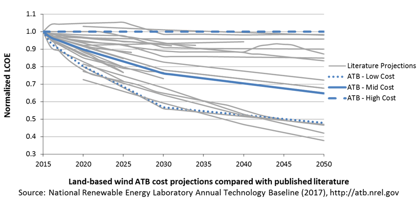
Expert survey estimates were normalized to the ATB Base Year starting point in order to focus on projected cost reduction instead of absolute reported costs. The percent reductions in LCOE by 2020, 2030, and 2050 from the expert survey's Median and Low scenarios are implemented as the ATB Mid and Low cost scenarios. This is accomplished by utilizing survey estimates for changes to capacity factor and O&M costs by 2030 and 2050. The corresponding CAPEX value to achieve the overall LCOE reduction is computed. The percent reduction in LCOE by 2030 and by 2050 was applied equally across all TRGs. The overall reduction in LCOE by 2050 for the Mid cost scenario is 35% and for the Low cost scenario is 53%.
A broad sample of cost of wind energy projections are shown to provide context for the ATB High, Mid, and Low cost projections. The ATB Mid cost projection, which corresponds to the Median scenario from the expert survey, results in LCOE reductions that are lower than median scenarios in the literature. The ATB Low cost projection, which corresponds to the Low scenario from the expert survey, is similar to the lower bound of the sample of literature projections.
Levelized Cost of Energy (LCOE) Projections
Levelized cost of energy (LCOE) is a simple metric that combines the primary technology cost and performance parameters, CAPEX, O&M, and capacity factor. It is included in the ATB for illustrative purposes. The focus of the ATB is to define the primary cost and performance parameters for use in electric sector modeling or other analysis where more sophisticated comparisons among technologies are made. LCOE captures the energy component of electric system planning and operation, but the electric system also requires capacity and flexibility services to operate reliably. Electricity generation technologies have different capabilities to provide such services. For example, wind and PV are primarily energy service providers, while the other electricity generation technologies provide capacity and flexibility services in addition to energy. These capacity and flexibility services are difficult to value and depend strongly on the system in which a new generation plant is introduced. These services are represented in electric sector models such as the ReEDS model and corresponding analysis results such as the Standard Scenarios.
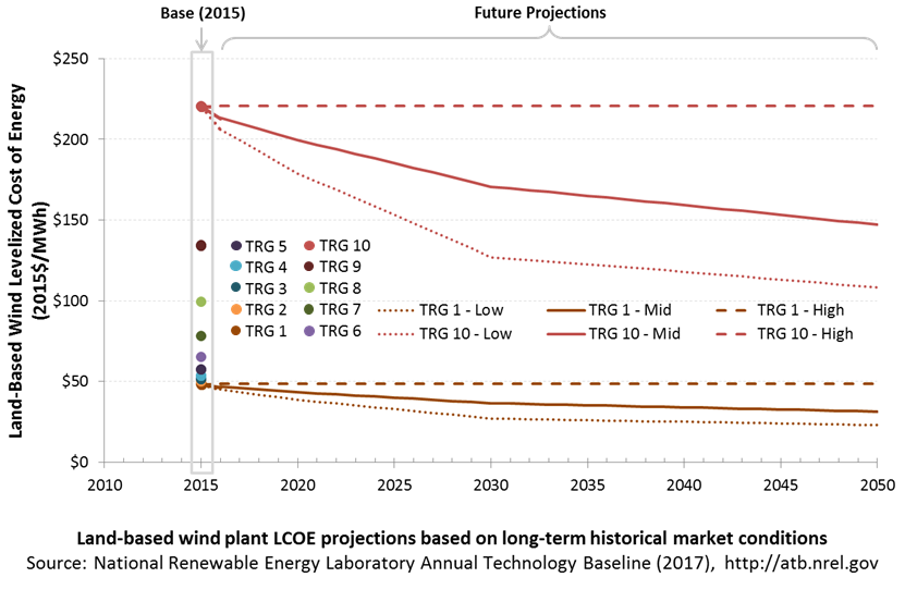
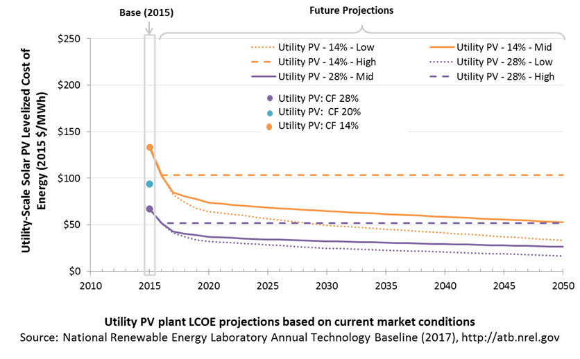
The following three figures illustrate the combined impact of CAPEX, O&M, and capacity factor projections across the range of resources present in the contiguous United States. The Current Market Conditions LCOE demonstrates the range of LCOE based on macroeconomic conditions similar to the present. The Historical Market Conditions LCOE presents the range of LCOE based on macroeconomic conditions consistent with prior ATB editions and Standard Scenarios model results. The Normalized LCOE (all LCOE estimates are normalized with the lowest Base Year LCOE value) emphasizes the effect of resource quality and the relative differences in the three future pathways independent of project finance assumptions. The ATB representative plant characteristics that best align with recently installed or anticipated near-term land-based wind plants are associated with TRG 4. Data for all the resource categories can be found in the ATB data spreadsheet.
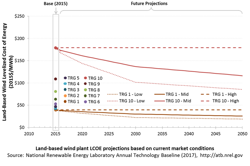
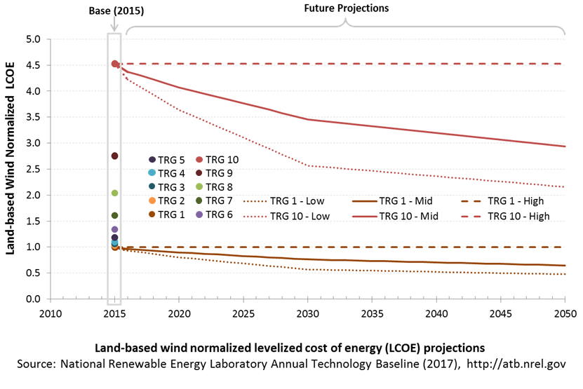
The methodology for representing the CAPEX, O&M, and capacity factor assumptions behind each pathway is discussed in Projections Methodology. The three pathways are generally defined as:
- High = Base Year (or near-term estimates of projects under construction) equivalent through 2050 maintains current relative technology cost differences
- Mid = technology advances through continued industry growth, public and private R&D investments, and market conditions relative to current levels that may be characterized as "likely" or "not surprising"
- Low = Technology advances that may occur with breakthroughs, increased public and private R&D investments, and/or other market conditions that lead to cost and performance levels that may be characterized as the "limit of surprise" but not necessarily the absolute low bound.
To estimate LCOE, assumptions about the cost of capital to finance electricity generation projects are required. For comparison in the ATB, two project finance structures are represented.
- Current Market Conditions: The values of the production tax credit (PTC) and investment tax credit (ITC) are ramping down by 2020, at which time wind and solar projects may be financed with debt fractions similar to other technologies. This scenario reflects debt interest (4.4% nominal, 1.9% real) and return on equity rates (9.5% nominal, 6.8% real) to represent 2017 market conditions (AEO 2017) and a debt fraction of 60% for all electricity generation technologies. An economic life, or period over which the initial capital investment is recovered, of 20 years is assumed for all technologies. These assumptions are one of the project finance options in the ATB spreadsheet.
- Long-Term Historical Market Conditions: Historically, debt interest and return on equity were represented with higher values. This scenario reflects debt interest (8% nominal, 5.4% real) and return on equity rates (13% nominal, 10.2% real) implemented in the ReEDS model and reflected in prior versions of the ATB and Standard Scenarios model results. A debt fraction of 60% for all electricity generation technologies is assumed. An economic life, or period over which the initial capital investment is recovered, of 20 years is assumed for all technologies. These assumptions are one of the project finance options in the ATB spreadsheet.
These parameters are held constant for estimates representing the Base Year through 2050. No incentives such as the PTC or ITC are included. The equations and variables used to estimate LCOE are defined on the equations and variables page. For illustration of the impact of changing financial structures such as WACC and economic life, see Project Finance Impact on LCOE. For LCOE estimates for High, Mid, and Low scenarios for all technologies, see 2017 ATB Cost and Performance Summary.
In general, the degree of adoption of a range of technology innovations distinguishes the High, Mid and Low cost cases. These projections represent the following trends to reduce CAPEX and FOM, and increase O&M.
- Continued turbine scaling to larger-megawatt turbines with larger rotors such that the swept area/megawatt capacity decreases, resulting in higher capacity factors for a given location
- Continued diversity of turbine technology whereby the largest rotor diameter turbines tend to be located in lower wind speed sites, but the number of turbine options for higher wind speed sites increases
- Taller towers that result in higher capacity factors for a given site due to the wind speed increase with elevation above ground level
- Improved plant siting and operation to reduce plant-level energy losses, resulting in higher capacity factors
- More efficient O&M procedures combined with more reliable components to reduce annual average FOM costs
- Continued manufacturing and design efficiencies such that capital cost/kilowatt decreases with larger turbine components
- Adoption of a wide range of innovative control, design, and material concepts that facilitate the above high-level trends.
Utility-Scale PV Power Plants
Representative Technology
Utility-scale PV systems in the ATB are representative of one-axis tracking systems with performance characteristics in line with a 1.1 DC-to-AC ratio - or inverter loading ratio (ILR) - and pricing characteristics in line with a 1.2 DC-to-AC ratio (Fu et al. 2016). PV system performance characteristics were designed in the ReEDS model at a time when PV system ILRs were lower than they are in current system designs; pricing in the 2017 ATB incorporates more up-to-date system designs and therefore assumes a higher ILR.
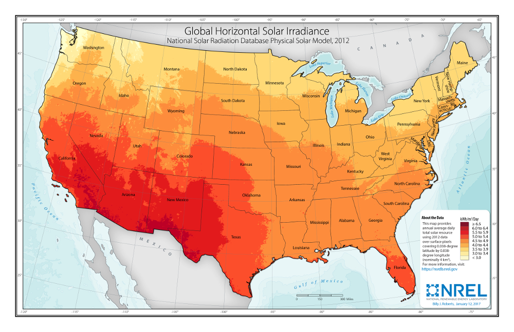
Resource Potential
Solar resources across the United States are mostly good to excellent at about 1,000-2,500 kWh/m2/year. The Southwest is at the top of this range, while Alaska and part of Washington are at the low end. The range for the contiguous United States is about 1,350-2,500 kWh/m2/year. Nationwide, solar resource levels vary by about a factor of two.
The total U.S. land area suitable for PV is significant and will not limit PV deployment. One estimate (Denholm and Margolis 2008) suggests the land area required to supply all end-use electricity in the United States using PV is about 5,500,000 hectares (ha) (13,600,000 acres), which is equivalent to 0.6% of the country's land area or about 22% of the "urban area" footprint (this calculation is based on deployment/land in all 50 states).
Renewable energy technical potential, as defined by Lopez et al. (2012), represents the achievable energy generation of a particular technology given system performance, topographic limitations, and environmental and land-use constraints. The primary benefit of assessing technical potential is that it establishes an upper-boundary estimate of development potential. It is important to understand that there are multiple types of potential - resource, technical, economic, and market (Lopez et al. 2012; NREL, "Renewable Energy Technical Potential").
Base Year and Future Year Projections Overview
The Base Year estimates rely on modeled CAPEX and O&M estimates benchmarked with industry and historical data. Capacity factor is estimated based on hours of sunlight at latitude for all geographic locations in the United States. The ATB presents capacity factor estimates that encompass a range associated with low, mid, and high levels across the United States.
Future year projections are derived from analysis of published projections of PV CAPEX and bottom-up engineering analysis of O&M costs. Three different projections were developed for scenario modeling as bounding levels:
- High cost: no change in CAPEX, O&M, or capacity factor from 2016 to 2050; consistent across all renewable energy technologies in the ATB
- Mid cost: based on the median of literature projections of future CAPEX; O&M technology pathway analysis
- Low Cost: based on low bound of literature projections of future CAPEX; O&M technology pathway analysis.
CAPital EXpenditures (CAPEX): Historical Trends, Current Estimates, and Future Projections
Capital expenditures (CAPEX) are expenditures required to achieve commercial operation in a given year. These expenditures include the hardware, the balance of system (e.g., site preparation, installation, and electrical infrastructure), and financial costs (e.g., development costs, onsite electrical equipment, and interest during construction) and are detailed in CAPEX Definition. In the ATB, CAPEX reflects typical plants and does not include differences in regional costs associated with labor or materials. The range of CAPEX demonstrates variation with resource in the contiguous United States.
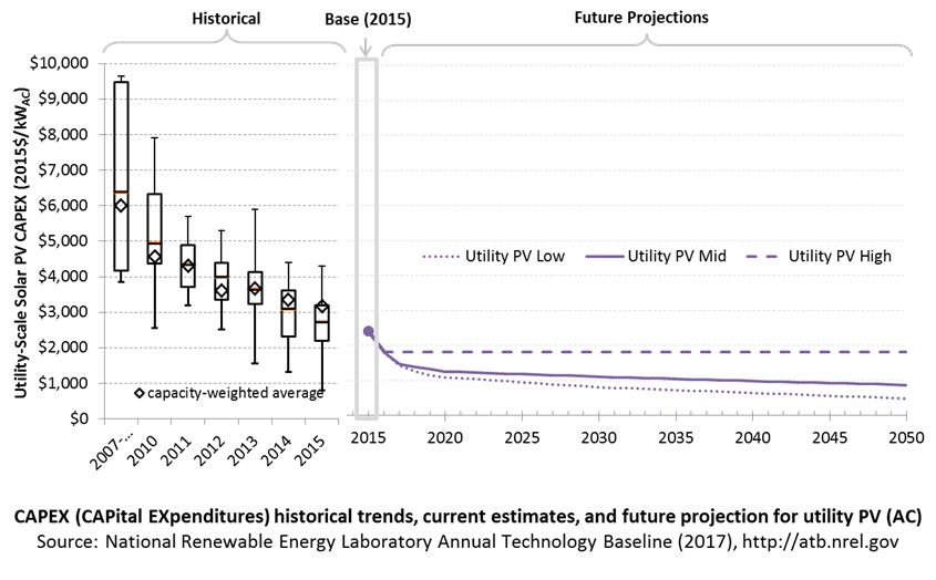
The following figures show the Base Year estimate and future year projections for CAPEX costs in terms of $/kWDC or $/kWAC. Three cost reduction scenarios are represented: High, Mid, and Low. Historical data from utility-scale PV plants installed in the United States are shown for comparison to the ATB Base Year estimates. The estimate for a given year represents CAPEX of a new plant that reaches commercial operation in that year.
The PV industry typically refers to PV CAPEX in terms of $/kWDC based on the aggregated module capacity. The electric utility industry typically refers to PV CAPEX in terms of $/kWAC based on the aggregated inverter capacity. See Solar PV AC-DC Translation for details. The figures illustrate the CAPEX historical trends, current estimates, and future projections in terms of $/kWDC or $/kWAC assuming an inverter loading ratio of 1.2.

Recent Trends
Reported historical utility-scale PV plant CAPEX (Bolinger and Seel 2016) is shown in box-and-whiskers format for comparison to the ATB current CAPEX estimates and future projections. Bolinger and Seel (2016) provide statistical representation of CAPEX for 89% of all utility-scale PV capacity.
PV pricing and capacities are quoted in kWDC (i.e., module rated capacity) unlike other generation technologies, which are quoted in kWAC. For PV, this would correspond to the combined rated capacity of all inverters. This is done because kWDC is the unit that the majority of the PV industry uses. Although costs are reported in kWDC, the total CAPEX includes the cost of the inverter, which has a capacity measured in kWAC.
CAPEX estimates for 2015 reflect continued rapid decline supported by analysis of recent power purchase agreement pricing (Bolinger and Seel 2016) for projects that will become operational in 2015 and beyond.
Base Year Estimates
For illustration in the ATB, a representative utility-scale PV plant is shown. Although the PV technologies vary, typical plant costs are represented with a single estimate because the CAPEX does not vary with solar resource.
Although the technology market share may shift over time with new developments, the typical plant cost is represented with the projections above.
A system price of $2.01/WDC in 2015 represents the median price of a utility-scale PV system installed in 2015 as reported in Bolinger and Seel (2016) and adjusted to remove regional cost multipliers based on geographic location of projects installed in 2015. The $1.51/WDC price in 2016 is based on modeled pricing for one-axis tracking systems quoted in Q1 2016 as reported in Fu et al. (2016) and adjusted for inflation. These figures are in line with other estimated system prices reported in Feldman et al. (2016).
The Base Year CAPEX estimates should tend toward the low end of reported pricing because no regional impacts, time-lagged system prices, or spur line costs are included. These effects are represented in the historical market data.
For example, in 2014, the reported capacity-weighted average system price was higher than 80% of system prices in 2014 due to very large systems, with multi-year construction schedules, installed in that year. Developers of these large systems negotiated contracts and installed portions of their systems when module and other costs were higher.
Future Year Projections
Projections of future utility-scale PV plant CAPEX are based on 14 system price projections from 8 separate institutions with short-term projections made in the past six months and long-term projections made in the last three years. We adjusted the "min," "median," and "max" analyst forecasts in a few different ways. All 2015 pricing is based on the median utility-scale system price as reported in Utility-Scale Solar 2015 (Bolinger and Seel 2016) and adjusted by the ReEDS state-level capital cost multipliers to remove geographic price distortions from 2015 reported pricing. All 2016 pricing is based on the bottom-up benchmark analysis reported in U.S. Solar Photovoltaic System Cost Benchmark Q1 2016 (adjusted for inflation) (Fu et al. 2016). These figures are in line with other estimated system prices reported in Feldman et al. (2016).
We adjusted the Mid and Low projections for 2017-2050 to remove distortions caused by the combination of forecasts with different time horizons and based on internal judgment of price trends. The High projection case is kept constant at the 2016 CAPEX value, assuming no improvements beyond 2016.
The largest annual reductions in CAPEX for the Mid and Low projections occur from 2015 to 2017, dropping 25% from 2015 to 2016 and another 19%-22% from 2016 to 2017. While reported CAPEX values have not been collected for all systems built in 2016 and 2017, CAPEX information collected from Annual Reports of Major Electric Utilities from the Federal Regulatory Commission (FERC Form 1) from nine major utilities found a 22% reduction in CAPEX from 2015 to 2016, falling to $1.32/W, which is well below reported CAPEX in the ATB. (FERC Form 1 collected from the FERC Online elibrary for the following utilities: Arizona Public Service, Florida Power & Light, Duke Energy Progressive, Georgia Power, Indiana Michigan Power Company, Kentucky Utilities, Pacific Gas & Electric, Public Service of New Mexico, and Southern California Edison.) The ATB values in 2017 are based on analysts' forecasts. Additionally, initially reported pricing for utility-scale power purchase agreements (PPAs) for utility-scale systems placed in service in that year fell 33% from 2015 to 2016; the ATB LCOE reduction over the same period is 23%.
Detailed description of the methodology for developing Future Year Projections is found in Projections Methodology.
Technology innovations that could impact future CAPEX costs are summarized in LCOE Projections.
CAPEX Definition
Capital expenditures (CAPEX) are expenditures required to achieve commercial operation in a given year.
For the ATB—and based on EIA (2016a) and the NREL Solar PV Cost Model (Fu et al. 2016) - the utility-scale solar PV plant envelope is defined to include:
- Hardware
- Module supply
- Power electronics, including inverters
- Racking
- Foundation
- AC and DC wiring materials and installation
- Electrical infrastructure, such as transformers, switchgear, and electrical system connecting modules to each other and to the control center
- Balance of system
- Land acquisition, site preparation, installation of underground utilities, access roads, fencing, and buildings for operations and maintenance
- Project indirect costs, including costs related to engineering, distributable labor and materials, construction management start up and commissioning, and contractor overhead costs, fees, and profit.
- Financial Costs
- Owner's costs, such as development costs, preliminary feasibility and engineering studies, environmental studies and permitting, legal fees, insurance costs, and property taxes during construction.
- Electrical interconnection, including onsite electrical equipment (e.g., switchyard), a nominal-distance spur line (<1 mile), and necessary upgrades at a transmission substation; distance-based spur line cost (GCC) not included in the ATB
- Interest during construction estimated based on six-month duration accumulated 100% at half-year intervals and an 8% interest rate (ConFinFactor).
CAPEX can be determined for a plant in a specific geographic location as follows:
CAPEX = ConFinFactor*(OCC*CapRegMult+GCC).
(See the Financial Definitions tab in the ATB data spreadsheet.)
Regional cost variations and geographically specific grid connection costs are not included in the ATB (CapRegMult = 1; GCC = 0). In the ATB, the input value is overnight capital cost (OCC) and details to calculate interest during construction (ConFinFactor).
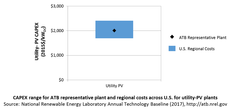
In the ATB, CAPEX represents a typical one-axis utility-scale PV plant and does not vary with resource. The difference in cost between tracking and non-tracking systems has been reduced greatly in the United States. Regional cost effects associated with labor rates, material costs, and other regional effects as defined by EIA (2016a) expand the range of CAPEX. Unique land-based spur line costs based on distance and transmission line costs for potential utility-PV plant locations expand the range of CAPEX even further. The following figure illustrates the ATB representative plant relative to the range of CAPEX including regional costs across the contiguous United States. The ATB representative plants are associated with a regional multiplier of 1.0.
Standard Scenarios Model Results
ATB CAPEX, O&M, and capacity factor assumptions for Base Year and future projections through 2050 for High, Mid, and Low projections are used to develop the NREL Standard Scenarios using the ReEDS model. See ATB and ATB and Standard Scenarios.
CAPEX in the ATB does not represent regional variants (CapRegMult) associated with labor rates, material costs, etc., but the ReEDS model does include 134 regional multipliers (EIA 2016a).
CAPEX in the ATB does not include a geographically determined spur line (GCC) from plant to transmission grid, but the ReEDS model calculates a unique value for each potential PV plant.
Operation and Maintenance (O&M) Costs
Operations and maintenance (O&M) costs represent the annual fixed expenditures required to operate and maintain a solar PV plant over its technical lifetime of 30 years (the distinction between economic life and technical life is described here), including:
- Insurance, property taxes, site security, legal and administrative fees, and other fixed costs
- Present value, annualized large component replacement costs over technical life (e.g., inverters at 15 years)
- Scheduled and unscheduled maintenance of solar PV plants, transformers, etc. over the technical lifetime of the plant (e.g., general maintenance, including cleaning and vegetation removal)
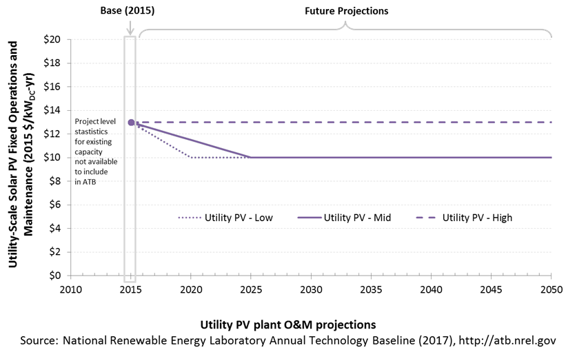
The following figure shows the Base Year estimate and future year projections for fixed O&M (FOM) costs. Three cost reduction scenarios are represented. The estimate for a given year represents annual average FOM costs expected over the technical lifetime of a new plant that reaches commercial operation in that year.
Base Year Estimates
FOM of $13/kWDC-yr is based on Bolinger and Seel (2016 ), who state that "average O&M costs for the cumulative set of PV plants within this sample have steadily declined from about $31/kWAC-yr (or $19/MWh) in 2011 to about $16/kWAC-yr ($7/MWh) in 2015." AC was converted into DC by dividing by 1.2. A wide range in reported prices exists in the market, in part depending on the maintenance practices that exist for a particular system. These cost categories include asset management (including compliance and reporting for incentive payments), different insurance products, site security, cleaning, vegetation removal, and failure of components. Not all these practices are performed for each system; additionally, some factors are dependent on the quality of the parts and construction. NREL analysts estimate O&M costs can range between $0 and $40/kWDC-yr.
Future Year Projections
Future FOM is assumed to decline to $10/kWDC-yr by 2020 in the Low cost case and by 2025 in the Mid cost case through improvements in system operation and more durable, better performing capital equipment, as per Woodhouse et al. 2016.
A detailed description of the methodology for developing future year projections is found in Projections Methodology.
Technology innovations that could impact future O&M costs are summarized in LCOE Projections.
Capacity Factor: Expected Annual Average Energy Production Over Lifetime
The capacity factor represents the expected annual average energy production divided by the annual energy production, assuming the plant operates at rated capacity for every hour of the year. It is intended to represent a long-term average over the technical lifetime of the plant (the distinction between economic life and technical life is described here). It does not represent interannual variation in energy production. Future year estimates represent the estimated annual average capacity factor over the technical lifetime of a new plant installed in a given year.
Other technologies' capacity factors are represented in exclusively AC units; however, because PV pricing in this ATB documentation is represented in $/kWDC, PV system capacity is a DC rating. The PV capacity factor is the ratio of annual average energy production (kWhAC) to annual energy production assuming the plant operates at rated DC capacity for every hour of the year. For more information, see Solar PV AC-DC Translation.
The capacity factor is influenced by the hourly solar profile, technology (e.g., thin-film versus crystalline silicon), axis type (e.g., none, one, or two), expected downtime, and inverter losses to transform from DC to AC power. The DC-AC ratio is a design choice that influences the capacity factor. PV plant capacity factor incorporates an assumed degradation rate of 0.5%/year (Jordan and Kurtz 2013) in the annual average calculation.
The following figure shows a range of capacity factors based on variation in solar resource in the contiguous United States. The range of the Base Year estimates illustrate the effect of locating a utility-scale PV plant in places with lower or higher solar irradiance. These values are the maximum, median, and minimum values for all geographic locations in the United States as implemented in the ReEDS model (Eurek et al. 2017 ). Future projections for High, Mid, and Low cost scenarios are unchanged from the Base Year. Technology improvements are focused on CAPEX and O&M cost elements.
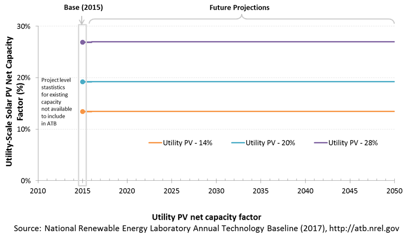
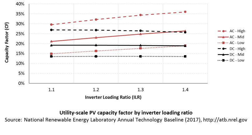
PV system inverters, which convert DC energy/power to AC energy/power, have AC capacity ratings; therefore, the capacity of a PV system is rated in MWAC, or the aggregation of all inverters' rated capacities, or MWDC, or the aggregation of all modules' rated capacities. The capacity factor calculation uses a system's rated capacity, and therefore, capacity factor can be represented using exclusively AC units or using AC units for electricity (the numerator) and DC units for capacity (the denominator). Both capacity factors will result in the same LCOE as long as the other variables use the same capacity rating (e.g., CAPEX in terms of $/kWDC). PV systems' DC ratings are typically higher than their AC ratings; therefore, the capacity factor calculated using a DC capacity rating has a higher denominator. In the ATB, we use capacity factors of 14%, 20%, and 28% for the first year of a PV project and adjust the values to reflect an average capacity factor for the lifetime of a project, calculated with MWDC, assuming 0.5% module capacity degradation per year. The adjusted average capacity factor values used in the ATB are 13.5%, 19.2%, and 26.9%. These numbers would change to approximately 14.8%, 21.2%, and 29.6% if the ATB used MWAC. The following figure illustrates capacity factor - both DC and AC - for a range of inverter loading ratios. The ATB capacity factor assumptions are based on ILR = 1.1.
Recent Trends
At the end of 2015, the capacity-weighted average AC capacity factor for all U.S. projects installed at the time was 27.6% (including fixed-tilt systems), but individual project-level capacity factors exhibited a wide range (15.1%–35.7%).
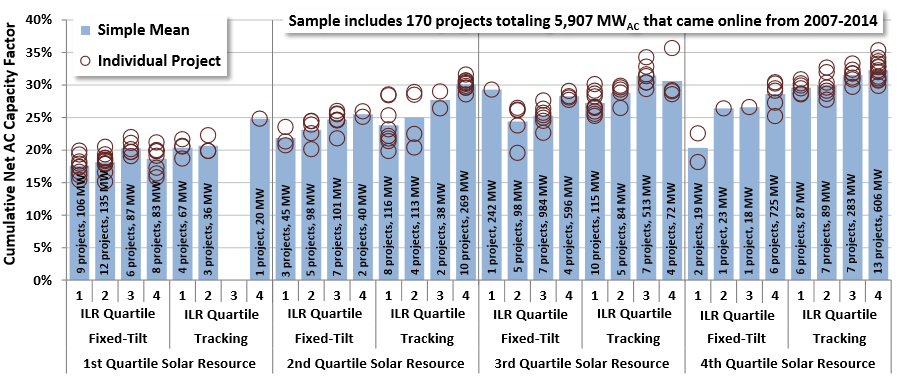
The capacity-weighted average capacity factor was more closely in line with the higher end of the range because 88% of the installed capacity was in the southwestern United States or California, where the average capacity factor was 30.2% for one-axis systems and 25.6% for fixed-tilt systems (Bolinger and Seel 2016). The upper and lower capacity factor values in the ATB are conservative due to the lower DC-to-AC ratio.
Base Year Estimates
For illustration in the ATB, a range of capacity factors associated with the range of latitude in the contiguous United States is shown.
Over time, PV plant output is reduced. This degradation (at 0.5%) is accounted for in ATB estimates of capacity factor. The ATB capacity factor estimates represent estimated annual average energy production over the 20-year economic life of the plant (the distinction between economic life and technical life is described here).
Given the historical reported capacity factors by systems installed in the United States and the potential for technological improvements that can improve the solar PV plant capacity factors (e.g., less reflectivity and improved low-light performance), these values likely represent a conservative estimate of system production. Part of this is due to differences in inverter loading ratios (also called DC-to-AC ratio), which can increase production but also increases cost ($/WDC). In 2015, the cumulative PV capacity factors for low-, mid-, and high-insolation regions, for tracking systems with a mid-level inverter loading ratio (1.19:1.25) were 20.7%, 26.7%, and 30.0% respectively (in WAC) (Bolinger and Seel 2016), which is comparable to or significantly higher than the 14.8%, 21.2%, and 29.6% (in WAC) used in the ATB (13.5%, 19.2%, and 26.9% in WDC). Currently reported capacity factors for deployed systems are, on average, reflective of capacity factors for relatively new plants.
These capacity factors are for a one-axis tracking system with a DC-to-AC ratio of 1.1.
Future Year Projections
Projections of capacity factors for plants installed in future years are unchanged from the Base Year. Solar PV plants have very little downtime, inverter efficiency is already optimized, and tracking is already assumed. That said, there is potential for future increases in capacity factors through technological improvements such as less panel reflectivity, lower degradation rates, and improved performance in low-light conditions.
Standard Scenarios Model Results
ATB CAPEX, O&M, and capacity factor assumptions for the Base Year and future projections through 2050 for High, Mid, and Low projections are used to develop the NREL Standard Scenarios using the ReEDS model. See ATB and Standard Scenarios.
The ReEDS model output capacity factors for wind and solar PV can be lower than input capacity factors due to endogenously estimated curtailments determined by system operation.
Plant Cost and Performance Projections Methodology
The capacity factor represents the assumed annual energy production divided by the total possible annual energy production, assuming the plant operates at rated capacity for every hour of the year. For biopower plants, the capacity factors are typically lower than their availability factors. Biopower plant availability factors have a wide range depending on system design, fuel type and availability, and maintenance schedules.
Biopower plants are typically baseload plants with steady capacity factors. For the ATB, the biopower capacity factor is taken as the average capacity factor for biomass plants for 2015, as reported by EIA.
Biopower capacity factors are influenced by technology and feedstock supply, expected downtime, and energy losses.

Levelized Cost of Energy (LCOE) Projections
Levelized cost of energy (LCOE) is a simple metric that combines the primary technology cost and performance parameters, CAPEX, O&M, and capacity factor. It is included in the ATB for illustrative purposes. The focus of the ATB is to define the primary cost and performance parameters for use in electric sector modeling or other analysis where more sophisticated comparisons among technologies are made. LCOE captures the energy component of electric system planning and operation, but the electric system also requires capacity and flexibility services to operate reliably. Electricity generation technologies have different capabilities to provide such services. For example, wind and PV are primarily energy service providers, while the other electricity generation technologies provide capacity and flexibility services in addition to energy. These capacity and flexibility services are difficult to value and depend strongly on the system in which a new generation plant is introduced. These services are represented in electric sector models such as the ReEDS model and corresponding analysis results such as the Standard Scenarios.
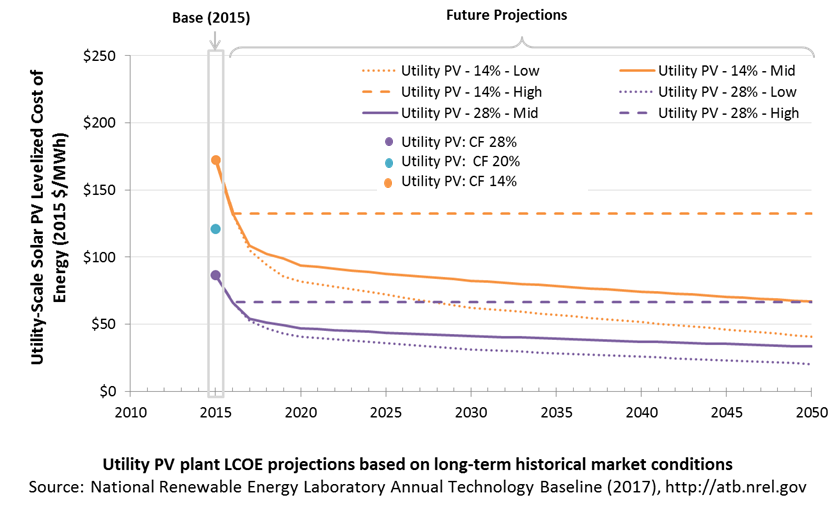
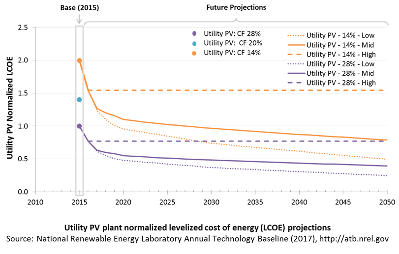
The following three figures illustrate the combined impact of CAPEX, O&M, and capacity factor projections across the range of resources present in the contiguous United States. The Current Market Conditions LCOE demonstrates the range of LCOE based on macroeconomic conditions similar to the present. The Historical Market Conditions LCOE presents the range of LCOE based on macroeconomic conditions consistent with prior ATB editions and Standard Scenarios model results. The Normalized LCOE (all LCOE estimates are normalized with the lowest Base Year LCOE value) emphasizes the effect of resource quality and the relative differences in the three future pathways independent of project finance assumptions. The ATB representative plant characteristics that best align with recently installed or anticipated near-term utility-scale PV plants are associated with Utility PV: CF 20%. Data for all the resource categories can be found in the ATB data spreadsheet.
The methodology for representing the CAPEX, O&M, and capacity factor assumptions behind each pathway is discussed in Projections Methodology. The three pathways are generally defined as:
- High = Base Year (or near-term estimates of projects under construction) equivalent through 2050 maintains current relative technology cost differences
- Mid = technology advances through continued industry growth, public and private R&D investments, and market conditions relative to current levels that may be characterized as "likely" or "not surprising"
- Low = Technology advances that may occur with breakthroughs, increased public and private R&D investments, and/or other market conditions that lead to cost and performance levels that may be characterized as the "limit of surprise" but not necessarily the absolute low bound.
To estimate LCOE, assumptions about the cost of capital to finance electricity generation projects are required. For comparison in the ATB, two project finance structures are represented.
- Current Market Conditions: The values of the production tax credit (PTC) and investment tax credit (ITC) are ramping down by 2020, at which time wind and solar projects may be financed with debt fractions similar to other technologies. This scenario reflects debt interest (4.4% nominal, 1.9% real) and return on equity rates (9.5% nominal, 6.8% real) to represent 2017 market conditions (AEO 2017) and a debt fraction of 60% for all electricity generation technologies. An economic life, or period over which the initial capital investment is recovered, of 20 years is assumed for all technologies. These assumptions are one of the project finance options in the ATB spreadsheet.
- Long-Term Historical Market Conditions: Historically, debt interest and return on equity were represented with higher values. This scenario reflects debt interest (8% nominal, 5.4% real) and return on equity rates (13% nominal, 10.2% real) implemented in the ReEDS model and reflected in prior versions of the ATB and Standard Scenarios model results. A debt fraction of 60% for all electricity generation technologies is assumed. An economic life, or period over which the initial capital investment is recovered, of 20 years is assumed for all technologies. These assumptions are one of the project finance options in the ATB spreadsheet.
These parameters are held constant for estimates representing the Base Year through 2050. No incentives such as the PTC or ITC are included. The equations and variables used to estimate LCOE are defined on the equations and variables page. For illustration of the impact of changing financial structures such as WACC and economic life, see Project Finance Impact on LCOE. For LCOE estimates for High, Mid, and Low scenarios for all technologies, see 2017 ATB Cost and Performance Summary.
In general, the degree of adoption of a range of technology innovations distinguishes the High, Mid and Low cost cases. These projections represent the following trends to reduce CAPEX and FOM.
- Modules
- Increased module efficiencies and increased production-line throughput to decrease CAPEX; overhead costs on a per-kilowatt will go down if efficiency and throughput improvement are realized.
- Reduced wafer thickness or the thickness of thin-film semiconductor layers
- Development of new semiconductor materials
- Development of larger manufacturing facilities in low-cost regions
- Balance of system (BOS)
- Increased module efficiency, reducing the size of the installation
- Development of racking systems that enhance energy production or require less robust engineering
- Integration of racking or mounting components in modules
- Reduction of supply chain complexity and cost
- Creation of standard packages system design
- Improvement supply chains for BOS components in modules
- Improved power electronics
- Improvement of inverter prices and performance, possibly by integrating micro-inverters
- Decreased installation costs and margins
- Reduction of supply chain margins (e.g., profit and overhead charged by suppliers, manufacturer, distributors, and retailers); this will likely occur naturally as the U.S. PV industry grows and matures.
- Streamlining of installation practices through improved workforce development and training, and developing standardized PV hardware
- Expansion of access to a range of innovative financing approaches and business models
- Development of best practices for permitting interconnection, and PV installation such as subdivision regulations, new construction guidelines, and design requirements.
FOM cost reduction represents optimized O&M strategies, reduced component replacement costs, and lower frequency of component replacement.
Geothermal
Hydrothermal Geothermal
Representative Technology
The typical geothermal plant size for hydrothermal resource sites is represented by a range of 30–40 MW, depending on the technology type (e.g., binary or flash) (Mines 2013).
Resource Potential
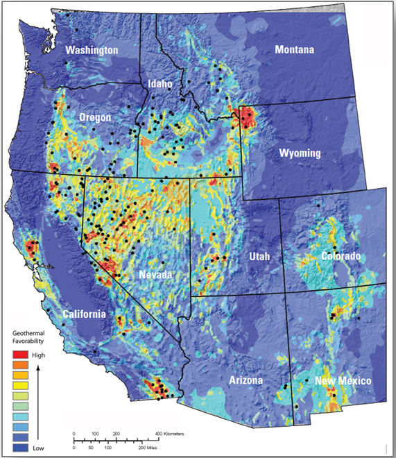
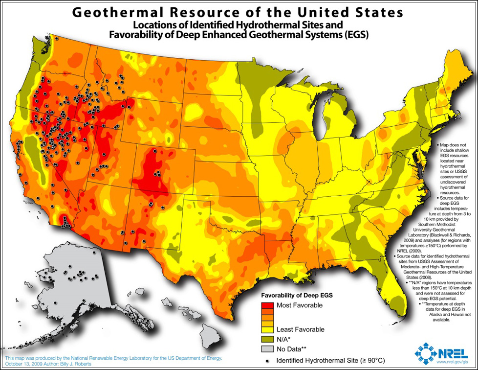
The hydrothermal geothermal resource is concentrated in the western United States. The total potential is 45,370 MW: 7,833 MW identified and 37,537 MW undiscovered (Williams et al. 2008). The U.S. Geological Survey (Williams et al. 2008) identified resource potential at each site is based on available reservoir thermal energy information from studies conducted at the site. The undiscovered hydrothermal technical potential estimate is based on a series of GIS statistical models for the spatial correlation of geological factors that facilitate the formation of geothermal systems.
The U.S. Geological Survey resource potential estimates for hydrothermal were used with the following modifications:
- Installed capacity of about 3 GW in 2014 is excluded from the resource potential
- Technical potential estimates increased 20%–30% to reflect impact of in-field enhanced geothermal system (EGS) technologies to increase (1) productivity of dry wells and (2) recovery of heat in place from hydrothermal reservoirs.
Renewable energy technical potential, as defined by Lopez et al. (2012), represents the achievable energy generation of a particular technology given system performance, topographic limitations, and environmental and land-use constraints. The primary benefit of assessing technical potential is that it establishes an upper-boundary estimate of development potential. It is important to understand that there are multiple types of potential-resource, technical, economic, and market (Lopez et al. 2012; NREL, "Renewable Energy Technical Potential").
Base Year and Future Year Projections Overview
The Base Year cost and performance estimates are calculated using Geothermal Electricity Technology Evaluation Model (GETEM), a bottom-up cost analysis tool that accounts for each phase of development of a geothermal plant (DOE "Geothermal Electricity Technology Evaluation Model").
- Cost and performance data for hydrothermal generation plants are estimated for each potential site using GETEM. Model results are based on resource attributes (e.g., estimated reservoir temperature, depth, and potential) of each site.
- Site attribute values are from Williams et al. (2008) for identified resource potential and from capacity-weighted averages of site attribute values of nearby identified resources for undiscovered resource potential.
- GETEM is used to estimate CAPEX, O&M, and parasitic plant losses that affect net energy production.
Projections of CAPEX for plants installed in future years are derived from minimum learning estimates (IEA 2017). Capacity factor and O&M costs for plants installed in future years are unchanged from the Base Year. Projections for hydrothermal and EGS technologies are equivalent.
- High cost: no change in CAPEX, O&M, or capacity factor from 2015 to 2050; consistent across all renewable energy technologies in the ATB
- Mid cost: CAPEX cost reduction based on half of assumed minimum learning
- Low cost: CAPEX cost reduction based on assumed minimum learning.
Enhanced Geothermal System (EGS) Technology
Representative Technology
The typical geothermal plant size for EGS plants is represented by a range of 20-25 MW for binary or flash technologies (Mines 2013).
Resource Potential
The enhanced geothermal system (EGS) resource is concentrated in the western United States. The total potential is greater than 100,000 MW: 1,493 MW of near-hydrothermal field EGS (NF-EGS) and the remaining potential comes from deep EGS.
- The NF-EGS resource potential is based on data from USGS for EGS potential on the periphery of select studied and identified hydrothermal sites.
- The deep EGS resource potential (Augustine 2011) is based on Southern Methodist University Geothermal Laboratory temp-at-depth maps and the methodology is from MIT (2006).
- The EGS resource is thousands of GW (16,000 GW) but many locations are likely not commercially feasible.
Renewable energy technical potential as defined by Lopez et al., (2012) represents the achievable energy generation of a particular technology given system performance, topographic limitations, environmental, and land-use constraints. The primary benefit of assessing technical potential is that it establishes an upper-boundary estimate of development potential. It is important to understand that there are multiple types of potential-resource, technical, economic, and market (Lopez et al. 2012; NREL, "Renewable Energy Technical Potential").
Base Year and Future Projections Overview
The Base Year cost and performance estimates are calculated using the Geothermal Electricity Technology Evaluation Model (GETEM), a bottom-up cost analysis tool that accounts for each phase of development of a geothermal plant (DOE "Geothermal Electricity Technology Evaluation Model").
- Cost and performance data for EGS generation plants are estimated for each potential site using GETEM. Model results based on resource attributes (e.g., estimated reservoir temperature, depth, and potential) of each site.
- Approaches to restrict resource potential to about 500 GW based on USGS analysis may be implemented in the future.
- GETEM is used to estimate CAPEX and O&M. and parasitic plant losses that affect net energy production.
Projections of CAPEX for plants installed in future years are derived from minimum learning estimates (IEA 2017). Capacity factor and O&M costs for plants installed in future years are unchanged from the Base Year. Projections for hydrothermal and enhanced geothermal system technologies are equivalent.
- High Cost: no change in CAPEX, O&M, or capacity factor from 2015 to 2050, consistent across all renewable energy technologies in the ATB
- Mid Cost: CAPEX cost reduction based on half of assumed minimum learning
- Low cost: CAPEX cost reduction based on assumed minimum learning.
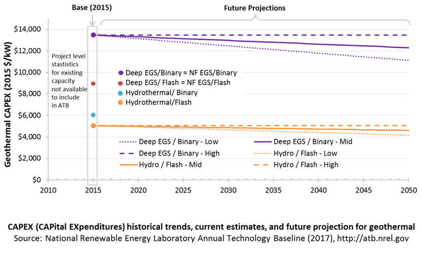
CAPital EXpenditures (CAPEX): Historical Trends, Current Estimates, and Future Projections
Capital expenditures (CAPEX) are expenditures required to achieve commercial operation in a given year. These expenditures include the geothermal generation plant, the balance of system (e.g., site preparation, installation, and electrical infrastructure), and financial costs (e.g., development costs, onsite electrical equipment, and interest during construction) and are detailed in CAPEX Definition. In the ATB, CAPEX reflects typical plants and does not include differences in regional costs associated with labor or materials. The range of CAPEX demonstrates variation with resource in the contiguous United States.
The following figure shows the Base Year estimate and future year projections for CAPEX costs. Three cost reduction scenarios are represented: High, Mid, and Low. The estimate for a given year represents CAPEX of a new plant that reaches commercial operation in that year.
Base Year Estimates
For illustration in the ATB, six representative geothermal plants are shown. Two energy conversion processes are common: binary organic Rankine cycle and flash.
- Binary plants use a heat exchanger to transfer geothermal energy to an organic Rankine cycle. This technology generally applies to lower-temperature systems. These systems have higher CAPEX than flash systems because of the increased number of components, their lower-temperature operation, and a general requirement that a number of wells be drilled for a given power output.
- Flash plants create steam directly from the thermal fluid through a pressure change. This technology generally applies to higher-temperature systems. Due to the reduced number of components and higher-temperature operation, these systems generally produce more power per well, thus reducing drilling costs. These systems generally have lower CAPEX than binary systems.
Examples using each of these plant types in each of the three resource types (hydrothermal, NF-EGS, and deep EGS) are shown in the ATB.
Costs are for new or "greenfield" hydrothermal projects, not for re-drilling or additional development/capacity additions at an existing site.
Characteristics for the six example plants representing current technology were developed based on discussion with industry stakeholders. The CAPEX estimates were generated using GETEM. CAPEX for NF-EGS and EGS are equivalent.
The table below shows the range of OCC associated with the resource characteristics for potential sites throughout the United States.
| Temp (°C) | |||||
|---|---|---|---|---|---|
| >=200C | 150–200 | 135–150 | <135 | ||
| Hydrothermal | |||||
| Number of identified sites | 21 | 23 | 17 | 59 | |
| Total capacity (MW) | 22,718 | 5,560 | 1,173 | 9,697 | |
| Avgerage OCC ($/kW) | 4,047 | 6,801 | 8,611 | 15,367 | |
| Min. OCC ($/kW) | 3,000 | 3,909 | 6,786 | 10,596 | |
| Max. OCC ($/kW) | 5,906 | 15,314 | 11,885 | 20,612 | |
| Example plant OCC ($/kW) | 4,567 | 5,465 | |||
| NF-EGS | Number of sites | 12 | 20 | ||
| Total capacity (MW) | 787 | 707 | |||
| Avgerage OCC ($/kW) | 5,928 | 8,820 | |||
| Min. OCC ($/kW) | 4,871 | 6,757 | |||
| Max. OCC ($/kW) | 7,216 | 11,486 | |||
| Example plant OCC ($/kW) | 8,100 | 12,179 | |||
| Deep EGS (3–6 km) | Number of sites | n/a | n/a | ||
| Total capacity (MW) | 100,000+ | ||||
| Average OCC ($/kW) | 10,061 | 20,840 | |||
| Min.OCC ($/kW) | 4,782 | 15,951 | |||
| Max. OCC ($/kW) | 18,292 | 25,933 | |||
| Example plant OCC ($/kW) | 8,100 | 12,179 | |||
Future Year Projections
Projection of future geothermal plant CAPEX for the Low case is based on minimum learning rates as implemented in AEO (EIA 2015): 10% by 2035. This corresponds to a 0.5% annual improvement in CAPEX, which is assumed to continue on through 2050. The Mid case is also considered with a 0.25% annual improvement in CAPEX through 2050.
A detailed description of the methodology for developing Future Year Projections is found in Projections Methodology.
Technology innovations that could impact future CAPEX costs are summarized in LCOE Projections.
CAPEX Definition
Capital expenditures (CAPEX) are expenditures required to achieve commercial operation in a given year.
For the ATB - and based on EIA (2016a) and GETEM component cost calculations - the geothermal plant envelope is defined to include:
- Geothermal generation plant
- Exploration, confirmation drilling, well field development, reservoir stimulation (EGS), plant equipment, and plant construction
- Power plant equipment, well-field equipment, and components for wells (including dry/non-commercial wells)
- Balance of system (BOS)
- Installation and electrical infrastructure, such as transformers, switchgear, and electrical system connecting turbines to each other and to the control center
- Project indirect costs, including costs related to engineering, distributable labor and materials, construction management start up and commissioning, and contractor overhead costs, fees, and profit
- Financial costs
- Owner's costs, such as development costs, preliminary feasibility and engineering studies, environmental studies and permitting, legal fees, insurance costs, and property taxes during construction
- Electrical interconnection and onsite electrical equipment (e.g., switchyard), a nominal-distance spur line (<1 mile), and necessary upgrades at a transmission substation; distance-based spur line cost (GCC) not included in the ATB
- Interest during construction estimated based on four-year duration accumulated 10%/20%/30%/40% at half-year intervals and an 8% interest rate (ConFinFactor).
CAPEX can be determined for a plant in a specific geographic location as follows:
CAPEX = ConFinFactor*(OCC*CapRegMult+GCC).
(See the Financial Definitions tab in the ATB data spreadsheet.)
Regional cost variations and geographically specific grid connection costs are not included in the ATB (CapRegMult = 1; GCC = 0). In the ATB, the input value is overnight capital cost (OCC) and details to calculate interest during construction (ConFinFactor).
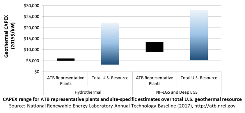
In the ATB, CAPEX is shown for six representative plants. Example CAPEX for binary organic Rankine cycle and flash energy conversion processes in each of three geothermal resource types are presented. CAPEX estimates for all hydrothermal NF-EGS potential results in a CAPEX range that is much broader than that shown in the ATB. It is unlikely that all of the resource potential will be developed due to the very high costs for some sites. Regional cost effects and distance-based spur line costs are not estimated.
Standard Scenarios Model Results
ATB CAPEX, O&M, and capacity factor assumptions for the Base Year and future projections through 2050 for High, Mid, and Low projections are used to develop the NREL Standard Scenarios using the ReEDS model. See ATB and Standard Scenarios.
The ReEDS model represents cost and performance for hydrothermal, NF-EGS, and EGS potential in 5 bins for each of 134 geographic regions, resulting in a greater CAPEX range in the reference supply curve than what is shown in examples in the ATB.
CAPEX in the ATB does not represent regional variants (CapRegMult) associated with labor rates, material costs, etc., and neither does the ReEDS model.
CAPEX in the ATB does not include geographically determined spur line (GCC) from plant to transmission grid, and neither does the ReEDS model.
Operation and Maintenance (O&M) Costs
Operations and maintenance (O&M) costs represent average annual fixed expenditures (and depend on rated capacity) required to operate and maintain a hydrothermal plant over its technical lifetime of 30 years (plant and reservoir) (the distinction between economic life and technical life is described here), including:
- Insurance, taxes, land lease payments, and other fixed costs
- Present value and annualized large component overhaul or replacement costs over technical life (e.g., downhole pumps)
- Scheduled and unscheduled maintenance of geothermal plant components and well field components over the technical lifetime of the plant and reservoir.
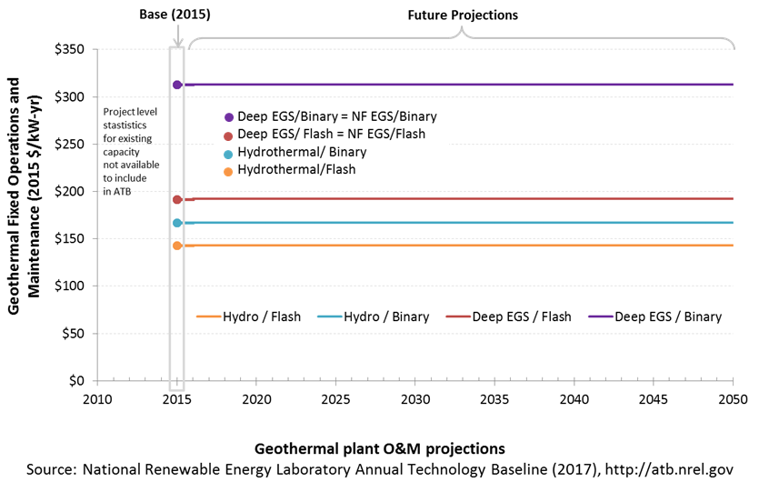
The following figure shows the Base Year estimate and future year projections for fixed O&M (FOM) costs. Three cost reduction scenarios are represented. The estimate for a given year represents annual average FOM costs expected over the technical lifetime of a new plant that reaches commercial operation in that year.
Base Year Estimates
FOM is estimated for each example plant based on technical characteristics.
GETEM is used to estimate FOM for each of the six representative plants. FOM for NF-EGS and EGS are equivalent.
Future Year Projections
No future FOM cost reduction is assumed in this edition of the ATB.
Capacity Factor: Expected Annual Average Energy Production Over Lifetime
The capacity factor represents the expected annual average energy production divided by the annual energy production, assuming the plant operates at rated capacity for every hour of the year. It is intended to represent a long-term average over the technical lifetime of the plant (the distinction between economic life and technical life is described here). It does not represent interannual variation in energy production. Future year estimates represent the estimated annual average capacity factor over the technical lifetime of a new plant installed in a given year.
Geothermal plant capacity factor is influenced by diurnal and seasonal air temperature variation (for air-cooled plants), technology (e.g., binary or flash), downtime, and internal plant energy losses.
The following figure shows a range of capacity factors based on variation in the resource for plants in the contiguous United States. The range of the Base Year estimates illustrates Binary or Flash geothermal plants. Future year projections for High, Mid, and Low cost scenarios are unchanged from the Base Year. Technology improvements are focused on CAPEX cost elements.
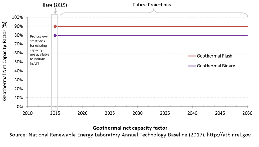
Base Year Estimate
The capacity factor estimates are developed using GETEM at typical design air temperature and based on design plant capacity net losses. An additional reduction is applied to approximate potential variability due to seasonal temperature effects.
Some geothermal plants have experienced year-on-year reductions in energy production, but this is not consistent across all plants. No approximation of long-term degradation of energy output is assumed.
Ongoing work at NREL and the Idaho National Laboratory is helping improve capacity factor estimates for geothermal plants. As this work progresses, it will be incorporated into future versions of the ATB.
Future Year Projections
Capacity factors remain unchanged from the Base Year through 2050. Technology improvements are focused on CAPEX costs. Estimates of capacity factor for geothermal plants in the ATB represent typical operation. The dispatch characteristics of these systems are valuable to the electric system to manage changes in net electricity demand. Actual capacity factors will be influenced by the degree to which system operators call on geothermal plants to manage grid services.
Plant Cost and Performance Projections Methodology
The site-specific nature of geothermal plant cost, the relative maturity of hydrothermal plant technology, and the very early stage development of EGS technologies make cost projections difficult. No thorough literature reviews have been conducted for cost reduction of hydrothermal geothermal technologies or EGS technologies. However, the Geothermal Vision Study, which is sponsored by the DOE Geothermal Technologies Office, is currently underway and is likely to lead to industry-developed cost reduction estimates that could be included in a future ATB..
Projection of future geothermal plant CAPEX for the Low cost case is based on minimum learning rates as implemented in AEO (EIA 2015): 10% by 2035. This corresponds to a 0.5% annual improvement in CAPEX, which is assumed to continue on through 2050. The Mid cost case assumes a 0.25% annual improvement in CAPEX through 2050. The High cost case retains all cost and performance assumptions equivalent to the Base Year through 2050.
Levelized Cost of Energy (LCOE) Projections
Levelized cost of energy (LCOE) is a simple metric that combines the primary technology cost and performance parameters, CAPEX, O&M, and capacity factor. It is included in the ATB for illustrative purposes. The focus of the ATB is to define the primary cost and performance parameters for use in electric sector modeling or other analysis where more sophisticated comparisons among technologies are made. LCOE captures the energy component of electric system planning and operation, but the electric system also requires capacity and flexibility services to operate reliably. Electricity generation technologies have different capabilities to provide such services. For example, wind and PV are primarily energy service providers, while the other electricity generation technologies provide capacity and flexibility services in addition to energy. These capacity and flexibility services are difficult to value and depend strongly on the system in which a new generation plant is introduced. These services are represented in electric sector models such as the ReEDS model and corresponding analysis results such as the Standard Scenarios.
The following three figures illustrate the combined impact of CAPEX, O&M, and capacity factor projections across the range of resources present in the contiguous United States. The Current Market Conditions LCOE demonstrates the range of LCOE based on macroeconomic conditions similar to the present. The Historical Market Conditions LCOE presents the range of LCOE based on macroeconomic conditions consistent with prior ATB editions and Standard Scenarios model results. The Normalized LCOE (all LCOE estimates are normalized with the lowest Base Year LCOE value) emphasizes the effect of resource quality and the relative differences in the three future pathways independent of project finance assumptions. The ATB representative plant characteristics that best align with recently installed or anticipated near-term geothermal plants are associated with Hydrothermal/Flash. Data for all the resource categories can be found in the ATB data spreadsheet.
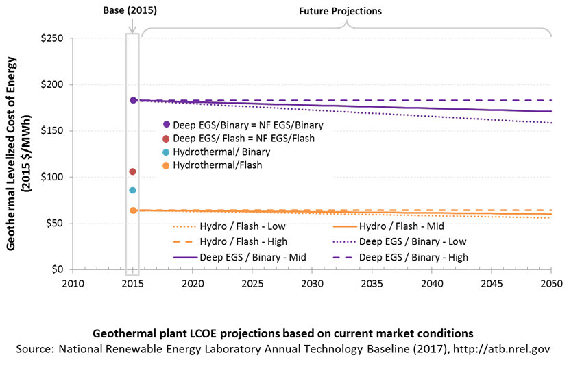
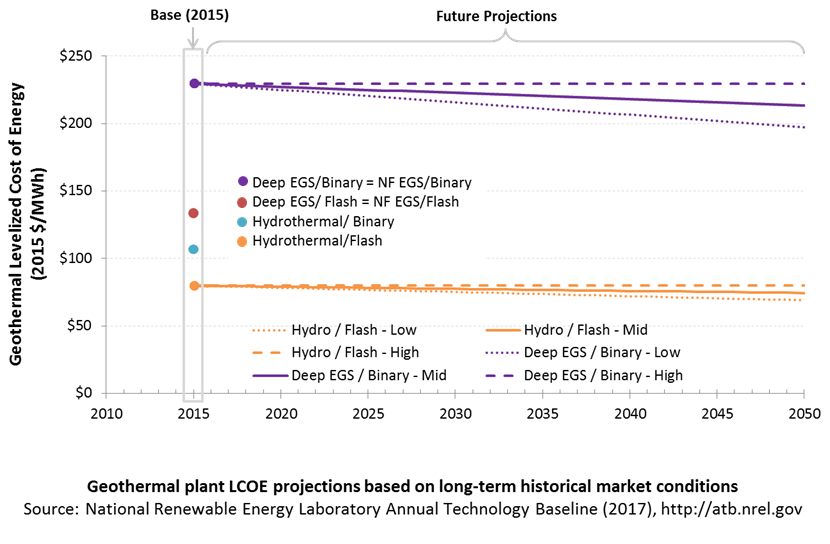
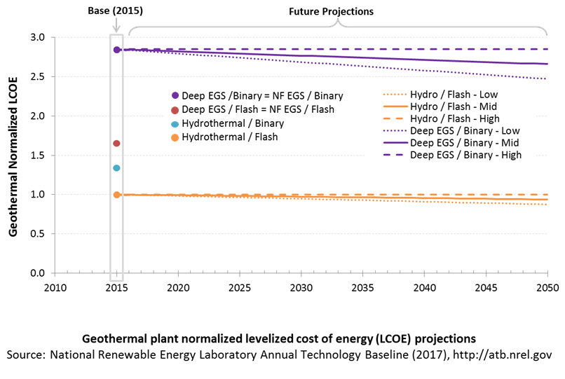
The methodology for representing the CAPEX, O&M, and capacity factor assumptions behind each pathway is discussed in Projections Methodology. The three pathways are generally defined as:
- High = Base Year (or near-term estimates of projects under construction) equivalent through 2050 maintains current relative technology cost differences
- Mid = Technology advances through continued industry growth, public and private R&D investments, and market conditions relative to current levels that may be characterized as "likely" or "not surprising"
- Low = Technology advances that may occur with breakthroughs, increased public and private R&D investments, and/or other market conditions that lead to cost and performance levels that may be characterized as the "limit of surprise" but not necessarily the absolute low bound.
To estimate LCOE, assumptions about the cost of capital to finance electricity generation projects are required. For comparison in the ATB, two project finance structures are represented.
- Current Market Conditions: The values of the production tax credit (PTC) and investment tax credit (ITC) are ramping down by 2020, at which time wind and solar projects may be financed with debt fractions similar to other technologies. This scenario reflects debt interest (4.4% nominal, 1.9% real) and return on equity rates (9.5% nominal, 6.8% real) to represent 2017 market conditions (AEO 2017) and a debt fraction of 60% for all electricity generation technologies. An economic life, or period over which the initial capital investment is recovered, of 20 years is assumed for all technologies. These assumptions are one of the project finance options in the ATB spreadsheet.
- Long-Term Historical Market Conditions: Historically, debt interest and return on equity were represented with higher values. This scenario reflects debt interest (8% nominal, 5.4% real) and return on equity rates (13% nominal, 10.2% real) implemented in the ReEDS model and reflected in prior versions of the ATB and Standard Scenarios model results. A debt fraction of 60% for all electricity generation technologies is assumed. An economic life, or period over which the initial capital investment is recovered, of 20 years is assumed for all technologies. These assumptions are one of the project finance options in the ATB spreadsheet.
These parameters are held constant for estimates representing the Base Year through 2050. No incentives such as the PTC or ITC are included. The equations and variables used to estimate LCOE are defined on the equations and variables page. For illustration of the impact of changing financial structures such as WACC and economic life, see Project Finance Impact on LCOE. For LCOE estimates for High, Mid, and Low scenarios for all technologies, see 2017 ATB Cost and Performance Summary.
Areas identified as having potential cost reduction opportunities include:
- Development of exploration and reservoir characterization tools that reduce well-field costs through risk reduction by locating and characterizing low- and moderate-temperature hydrothermal systems prior to drilling
- High-temperature tools and electronics for geothermal subsurface operations
- Novel or mixed working fluids in binary power plant designed to increase plant efficiency
- Advanced drilling systems such as using flames or lasers to drill through rock; drilling steering technology; and other technologies to reduce drilling costs.
Natural Gas Plants
A gas-fired combustion turbine involves:
- An air compressor compresses air and feeds it into the combustion chamber at hundreds of miles per hour.
- In a combustion system, a ring of fuel injectors inject fuel into combustion chambers where it mixes with the air and is combusted. The resulting high-temperature, high-pressure gas stream enters and expands through the turbine.
- A turbine has alternate stationary and rotating airfoil-section blades that are driven by expanding hot combustion gas. The rotating blades drive the compressor and spin a generator to produce electricity.
Simple-cycle gas turbines can achieve 20%-35% energy conversion efficiency depending on the type and design of the system. Aeroderivative turbines are typically more flexible but more expensive than their industrial gas turbine counterparts. Combined-cycle natural gas plants include a heat recovery steam generator that uses the hot exhaust from the combustion turbine to generate steam. That steam can then be used to generate additional electricity using a steam turbine. Combined-cycle natural gas plants typically have efficiencies ranging from 50%-60%, and R&D targets have been set to achieve even higher efficiencies. Combined-cycle plants can be built using a variety of configurations, such as a single combustion turbine and steam turbine connected to a single generator (1x1) or two combustion turbines coupled with one steam turbine (2x1) (DOE "How Gas Turbine Power Plants Work").
Renewable energy technical potential, as defined by Lopez et al. (2012), represents the achievable energy generation of a particular technology given system performance, topographic limitations, and environmental and land-use constraints. Technical resource potential corresponds most closely to fossil reserves, as both can be characterized by the prospect of commercial feasibility and depend strongly on available technology at the time of the resource assessment. Natural gas reserves in the United States are assessed by the United States Geological Survey (USGS, "National Oil and Gas Assessment").
This section focuses on large, utility-scale natural gas plants. Distributed-scale turbines may be included in a future version of the ATB.
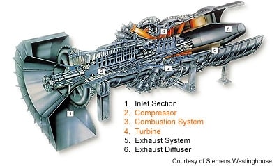
CAPital EXpenditures (CAPEX): Historical Trends, Current Estimates, and Future Projections
Because natural gas plants are well-known and perform close to their optimal performance, the EIA capital expenditures (CAPEX) projections decline at the minimum learning rate for the gas-fired technologies, resulting in incremental improvement over time that progresses slightly more quickly than inflation.
The one exception is natural gas combined cycle (CC) with carbon capture and storage (CCS). The DOE Office of Fossil Energy and the National Energy Technology Laboratory conduct research on reducing the costs and increasing the performance of CCS technology, and costs are expected to decline over time at a higher learning rate than the more mature gas-CT and gas-CC technologies.
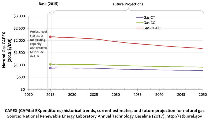
Comparison with Other Sources
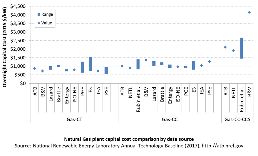
Costs vary due to differences in configuration (e.g., 2x1 versus 1x1), turbine class, and methodology. All costs were converted to the same dollar year.
CAPEX Definition
Capital expenditures (CAPEX) are expenditures required to achieve commercial operation in a given year.
Overnight capital costs are modified from EIA (2017). Capital costs include overnight capital cost plus defined transmission cost, and it removes a material price index.
Fuel costs are taken from EIA (2017). EIA reports two types of gas-CT and gas-CC technologies in the Annual Energy Outlook: advanced (H-class for gas-CC, F-class for gas-CT) and conventional (F-class for gas-CC, LM-6000 for gas-CT). Because we represent a single gas-CT and gas-CC technology in the ATB, the characteristics for the ATB plants are taken to be the average of the advanced and conventional systems as reported by EIA. For example, the OCC for the gas-CC technology in the ATB is the average of the capital cost of the advanced and conventional combined cycle technologies from the EIA's Annual Energy Outlook. Future work aims to improve the representation of the various natural gas technologies in the ATB. The CCS plant configuration includes only the cost of capturing and compressing the CO2. It does not include CO2 delivery and storage.
| Overnight Capital Cost ($/kW) | Construction Financing Factor (ConFinFactor) | CAPEX ($/kW) | |
|---|---|---|---|
| Gas-CT: Conventional combustion turbine | $864 | 1.021 | $882 |
| Gas-CC: Conventional combined cycle | $1,010 | 1.021 | $1,032 |
| Gas-CC-CCS: Combined cycle with carbon capture sequestration | $2,109 | 1.021 | $2,154 |
CAPEX can be determined for a plant in a specific geographic location as follows:
CAPEX = ConFinFactor × (OCC×CapRegMult+GCC).
(See the Financial Definitions tab in the ATB data spreadsheet.)
Regional cost variations and geographically specific grid connection costs are not included in the ATB (CapRegMult=1; GCC=0). In the ATB, the input value is overnight capital cost (OCC) and details to calculate interest during construction (ConFinFactor).
In the ATB, CAPEX represents each type of gas plant with a unique value. Regional cost effects associated with labor rates, material costs, and other regional effects as defined by EIA (2016a) expand the range of CAPEX. Unique land-based spur line costs based on distance and transmission line costs are not estimated. The following figure illustrates the ATB representative plant relative to the range of CAPEX including regional costs across the contiguous United States. The ATB representative plants are associated with a regional multiplier of 1.0.
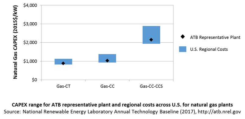
Operation and Maintenance (O&M) Costs
Operations and maintenance (O&M) costs represent the annual expenditures required to operate and maintain a plant over its technical lifetime (the distinction between economic life and technical life is described here), including:
- Insurance, taxes, land lease payments, and other fixed costs
- Present value and annualized large component replacement costs over technical life
- Scheduled and unscheduled maintenance of power plants, transformers, and other components over the technical lifetime of the plant.
Market data for comparison are limited and generally inconsistent in the range of costs covered and the length of the historical record.
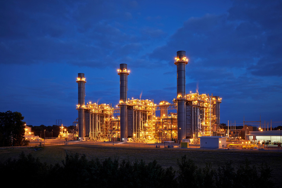
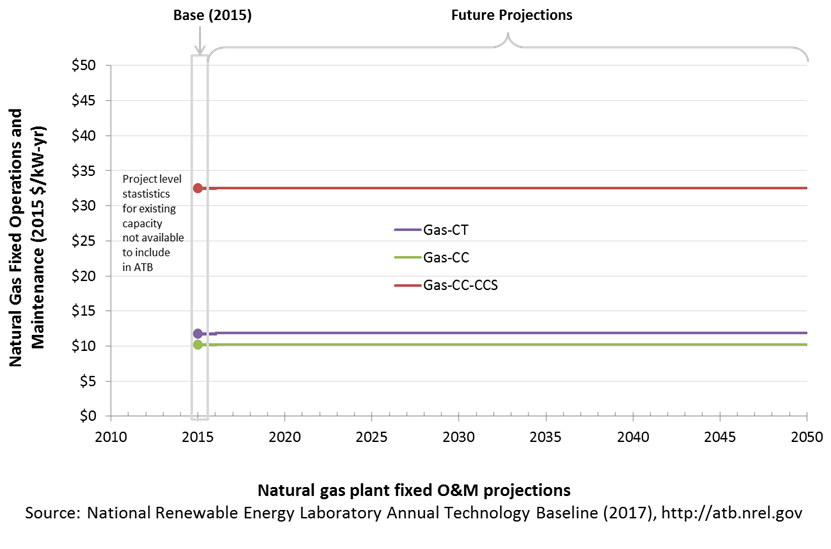
Capacity Factor: Expected Annual Average Energy Production Over Lifetime
The capacity factor represents the assumed annual energy production divided by the total possible annual energy production, assuming the plant operates at rated capacity for every hour of the year. For natural gas plants, the capacity factor is typically lower (and, in the case of combustion turbines, much lower) than their availability factor. Natural gas plants have availability factors approaching 100%.
The capacity factors of dispatchable units is typically a function of the unit's marginal costs and local grid needs (e.g., need for voltage support or limits due to transmission congestion). The average capacity factor is the average fleet-wide capacity factor for these plant types in 2015. The high capacity factor is taken from EIA (2016c, Table 1a) for a new power plant and represents a high bound of operation for a plant of this type.
Gas-CT power plants are less efficient than gas-CC power plants, and they tend to run as intermediate or peaker plants.
Gas-CC with CCS has not yet been built. It is expected to be a baseload unit.
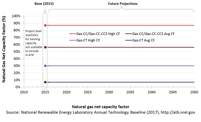
Levelized Cost of Energy (LCOE) Projections
Levelized cost of energy (LCOE) is a simple metric that combines the primary technology cost and performance parameters, CAPEX, O&M, and capacity factor. It is included in the ATB for illustrative purposes. The focus of the ATB is to define the primary cost and performance parameters for use in electric sector modeling or other analysis where more sophisticated comparisons among technologies are made. LCOE captures the energy component of electric system planning and operation, but the electric system also requires capacity and flexibility services to operate reliably. Electricity generation technologies have different capabilities to provide such services. For example, wind and PV are primarily energy service providers, while the other electricity generation technologies provide capacity and flexibility services in addition to energy. These capacity and flexibility services are difficult to value and depend strongly on the system in which a new generation plant is introduced. These services are represented in electric sector models such as the ReEDS model and corresponding analysis results such as the Standard Scenarios.
The following three figures illustrate the combined impact of CAPEX, O&M, and capacity factor projections across the range of resources present in the contiguous United States. The Current Market Conditions LCOE demonstrates the range of LCOE based on macroeconomic conditions similar to the present. The Historical Market Conditions LCOE presents the range of LCOE based on macroeconomic conditions consistent with prior ATB editions and Standard Scenarios model results. The Normalized LCOE (all LCOE estimates are normalized with the lowest Base Year LCOE value) emphasizes the relative effect of fuel price and heat rate independent of project finance assumptions. The ATB representative plant characteristics that best align with recently installed or anticipated near-term natural gas plants are associated with Gas-CC-HighCF. Data for all the resource categories can be found in the ATB data spreadsheet.
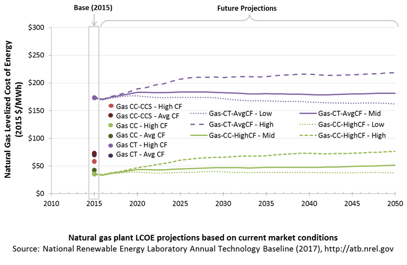
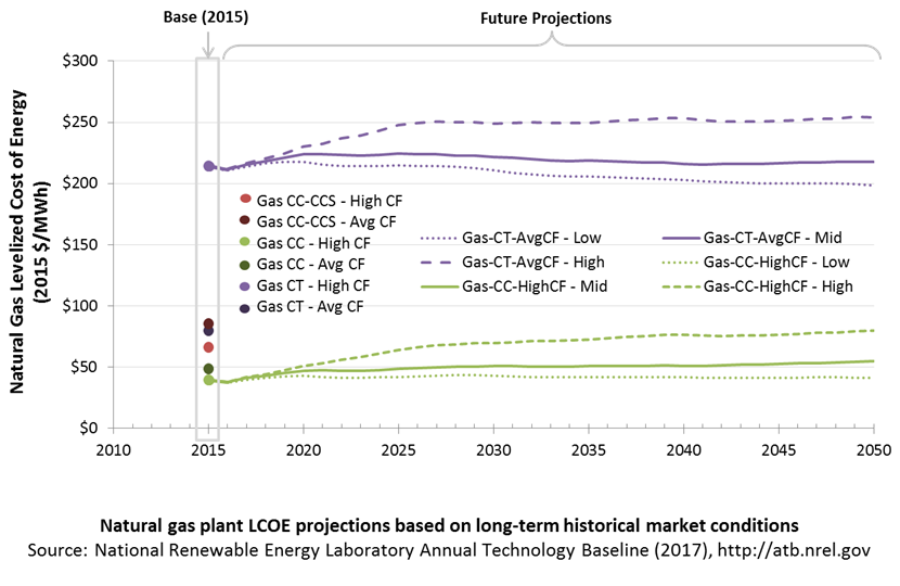
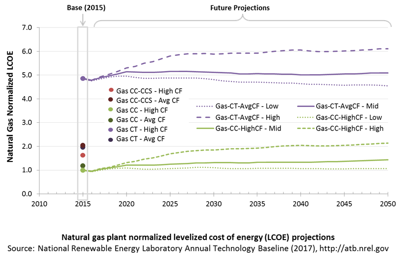
The LCOE of natural gas plants is directly impacted by the price of the natural gas fuel, so we include low, median, and high natural gas price trajectories. The LCOE is also impacted by variations in the heat rate and O&M costs. Because the reference and high natural gas price projections from AEO 2017 are rising over time, the LCOE of new natural gas plants can actually increase over time if the gas prices rise faster than the capital costs decline. For a given year, the LCOE assumes that the fuel prices from that year continue throughout the lifetime of the plant.
These projections do not include any cost of carbon, which would influence the LCOE of fossil units. Also, for CCS plants, the potential revenue from selling the captured carbon is not included (e.g., enhanced oil recovery operation may purchase CO2 from a CCS plant).
Fuel prices are based on the EIA's Annual Energy Outlook 2017 (EIA 2017).
To estimate LCOE, assumptions about the cost of capital to finance electricity generation projects are required. For comparison in the ATB, two project finance structures are represented.
- Current Market Conditions: The values of the production tax credit (PTC) and investment tax credit (ITC) are ramping down by 2020, at which time wind and solar projects may be financed with debt fractions similar to other technologies. This scenario reflects debt interest (4.4% nominal, 1.9% real) and return on equity rates (9.5% nominal, 6.8% real) to represent 2017 market conditions (AEO 2017) and a debt fraction of 60% for all electricity generation technologies. An economic life, or period over which the initial capital investment is recovered, of 20 years is assumed for all technologies. These assumptions are one of the project finance options in the ATB spreadsheet.
- Long-Term Historical Market Conditions: Historically, debt interest and return on equity were represented with higher values. This scenario reflects debt interest (8% nominal, 5.4% real) and return on equity rates (13% nominal, 10.2% real) implemented in the ReEDS model and reflected in prior versions of the ATB and Standard Scenarios model results. A debt fraction of 60% for all electricity generation technologies is assumed. An economic life, or period over which the initial capital investment is recovered, of 20 years is assumed for all technologies. These assumptions are one of the project finance options in the ATB spreadsheet.
These parameters are held constant for estimates representing the Base Year through 2050. No incentives such as the PTC or ITC are included. The equations and variables used to estimate LCOE are defined on the equations and variables page. For illustration of the impact of changing financial structures such as WACC and economic life, see Project Finance Impact on LCOE. For LCOE estimates for High, Mid, and Low scenarios for all technologies, see 2017 ATB Cost and Performance Summary.
Biopower Plants
In a biopower plant:
- Heat is created: Biomass (sometimes co-fired with coal) is pulverized, mixed with hot air, and burned in suspension.
- Water turns to steam: The heat turns purified water into steam, which is piped to the turbine.
- Steam turns the turbine: The pressure of the steam pushes the turbine blade, turns the shaft in the generator, and creates power.
- Steam is turned back into water: Cool water is drawn into a condenser where the steam turns back into water that can be reused in the plant.
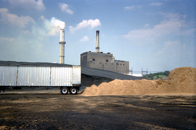
(a biomass gasifier that operates on wood chips)
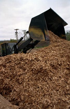
Renewable energy technical potential, as defined by Lopez et al. (2012), represents the achievable energy generation of a particular technology given system performance, topographic limitations, and environmental and land-use constraints. Technical resource potential for biopower is based on estimated biomass quantities from the Billion Ton Update study (DOE 2011).
CAPital EXpenditures (CAPEX): Historical Trends, Current Estimates, and Future Projections
Because biopower plants are well-known and perform close to their optimal performance, EIA expects capital expenditures (CAPEX) will incrementally improve over time and slightly more quickly than inflation.
The exception is new biomass cofiring, which is expected to have costs that decline a bit more than existing cofiring project technologies.
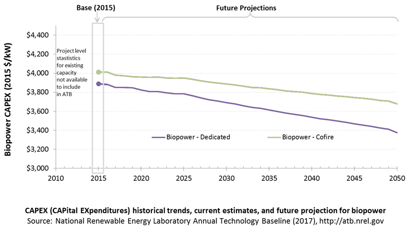
CAPEX Definition
Capital expenditures (CAPEX) are expenditures required to achieve commercial operation in a given year.
Overnight capital costs are modified from EIA (2014). Capital costs include overnight capital cost plus defined transmission cost, and it removes a material price index. The overnight capital costs for cofired units are not the cost of upgrading a plant but the total cost of the plant after the upgrade.
Fuel costs are taken from the Billion Ton Update study (DOE 2011).
| Overnight Capital Cost ($/kW) | Construction Financing Factor (ConFinFactor) | CAPEX ($/kW) | |
|---|---|---|---|
| Dedicated: Dedicated biopower plant | $3,737 | 1.041 | $3,889 |
| CofireOld: Pulverized coal with sulfur dioxide (SO2) scrubbers and biomass co-firing | $3,856 | 1.041 | $4,013 |
| CofireNew: Advanced supercritical coal with SO2 and NOx controls and biomass co-firing | $3,856 | 1.041 | $4,013 |
CAPEX can be determined for a plant in a specific geographic location as follows:
CAPEX = ConFinFactor*(OCC*CapRegMult+GCC).
(See the Financial Definitions tab in the ATB data spreadsheet.)
Regional cost variations and geographically specific grid connection costs are not included in the ATB (CapRegMult = 1; GCC = 0). In the ATB, the input value is overnight capital cost (OCC) and details to calculate interest during construction (ConFinFactor).
In the ATB, CAPEX represents each type of biopower plant with a unique value. Regional cost effects associated with labor rates, material costs, and other regional effects as defined by EIA (2016a) expand the range of CAPEX. Unique land-based spur line costs based on distance and transmission line costs are not estimated. The following figure illustrates the ATB representative plant relative to the range of CAPEX including regional costs across the contiguous United States. The ATB representative plants are associated with a regional multiplier of 1.0.
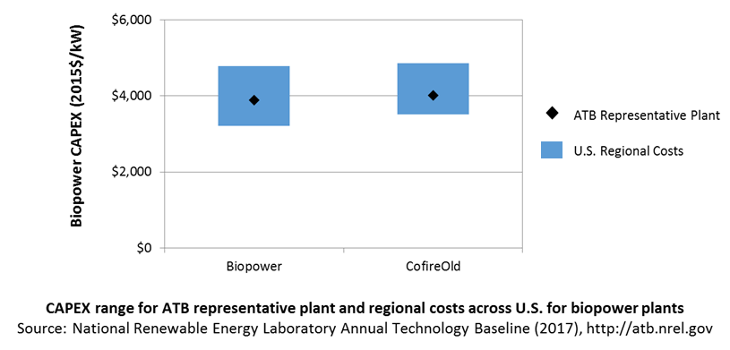
Operation and Maintenance (O&M) Costs
Operations and maintenance (O&M) costs represent the annual expenditures required to operate and maintain a plant over its technical lifetime (the distinction between economic life and technical life is described here), including:
- Insurance, taxes, land lease payments, and other fixed costs
- Present value and annualized large component replacement costs over technical life
- Scheduled and unscheduled maintenance of power plants, transformers, and other components over the technical lifetime of the plant.
Market data for comparison are limited and generally inconsistent in the range of costs covered and the length of the historical record.
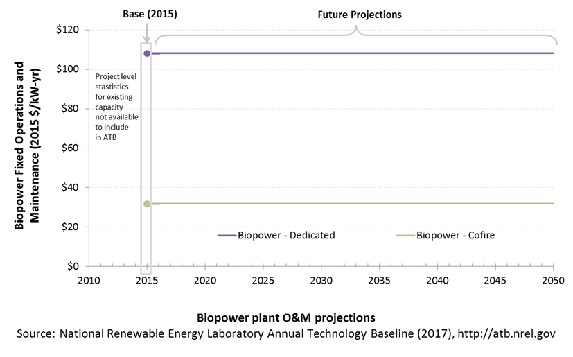
Capacity Factor: Expected Annual Average Energy Production Over Lifetime
The capacity factor represents the assumed annual energy production divided by the total possible annual energy production, assuming the plant operates at rated capacity for every hour of the year. For biopower plants, the capacity factors are typically lower than their availability factors. Biopower plant availability factors have a wide range depending on system design, fuel type and availability, and maintenance schedules.
Biopower plants are typically baseload plants with steady capacity factors. For the ATB, the biopower capacity factor is taken as the average capacity factor for biomass plants for 2015, as reported by EIA.
Biopower capacity factors are influenced by technology and feedstock supply, expected downtime, and energy losses.
Levelized Cost of Energy (LCOE) Projections
Levelized cost of energy (LCOE) is a simple metric that combines the primary technology cost and performance parameters, CAPEX, O&M, and capacity factor. It is included in the ATB for illustrative purposes. The focus of the ATB is to define the primary cost and performance parameters for use in electric sector modeling or other analysis where more sophisticated comparisons among technologies are made. LCOE captures the energy component of electric system planning and operation, but the electric system also requires capacity and flexibility services to operate reliably. Electricity generation technologies have different capabilities to provide such services. For example, wind and PV are primarily energy service providers, while the other electricity generation technologies provide capacity and flexibility services in addition to energy. These capacity and flexibility services are difficult to value and depend strongly on the system in which a new generation plant is introduced. These services are represented in electric sector models such as the ReEDS model and corresponding analysis results such as the Standard Scenarios.
The following three figures illustrate the combined impact of CAPEX, O&M, and capacity factor projections across the range of resources present in the contiguous United States. The Current Market Conditions LCOE demonstrates the range of LCOE based on macroeconomic conditions similar to the present. The Historical Market Conditions LCOE presents the range of LCOE based on macroeconomic conditions consistent with prior ATB editions and Standard Scenarios model results. The Normalized LCOE (all LCOE estimates are normalized with the lowest Base Year LCOE value) emphasizes the relative effect of fuel price and heat rate independent of project finance assumptions. Data for all the resource categories can be found in the ATB data spreadsheet.
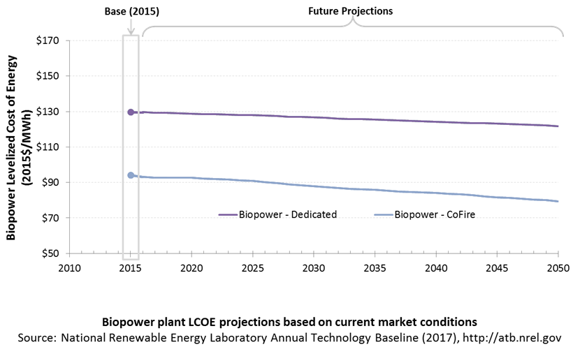
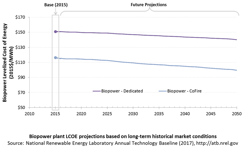
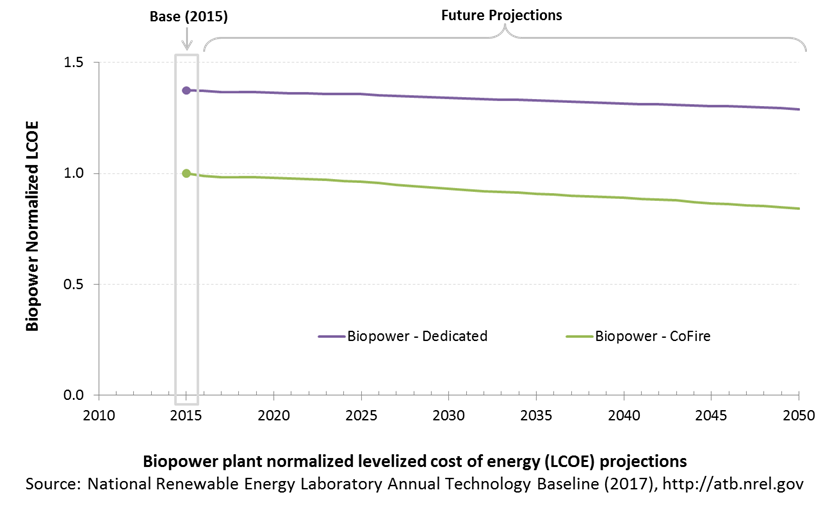
The LCOE of biopower plants is directly impacted by the differences in CAPEX (installed capacity costs) as well as by heat rate differences. For a given year, the LCOE assumes that the fuel prices from that year continue throughout the lifetime of the plant.
Regional variations will ultimately impact biomass feedstock costs, but these are not included in the ATB.
The projections do not include any cost of carbon.
Fuel prices are based on the EIA's Annual Energy Outlook 2017 (EIA 2017).
To estimate LCOE, assumptions about the cost of capital to finance electricity generation projects are required. For comparison in the ATB, two project finance structures are represented.
- Current Market Conditions: The values of the production tax credit (PTC) and investment tax credit (ITC) are ramping down by 2020, at which time wind and solar projects may be financed with debt fractions similar to other technologies. This scenario reflects debt interest (4.4% nominal, 1.9% real) and return on equity rates (9.5% nominal, 6.8% real) to represent 2017 market conditions (AEO 2017) and a debt fraction of 60% for all electricity generation technologies. An economic life, or period over which the initial capital investment is recovered, of 20 years is assumed for all technologies. These assumptions are one of the project finance options in the ATB spreadsheet.
- Long-Term Historical Market Conditions: Historically, debt interest and return on equity were represented with higher values. This scenario reflects debt interest (8% nominal, 5.4% real) and return on equity rates (13% nominal, 10.2% real) implemented in the ReEDS model and reflected in prior versions of the ATB and Standard Scenarios model results. A debt fraction of 60% for all electricity generation technologies is assumed. An economic life, or period over which the initial capital investment is recovered, of 20 years is assumed for all technologies. These assumptions are one of the project finance options in the ATB spreadsheet.
These parameters are held constant for estimates representing the Base Year through 2050. No incentives such as the PTC or ITC are included. The equations and variables used to estimate LCOE are defined on the equations and variables page. For illustration of the impact of changing financial structures such as WACC and economic life, see Project Finance Impact on LCOE. For LCOE estimates for High, Mid, and Low scenarios for all technologies, see 2017 ATB Cost and Performance Summary.
References
Augustine, C. 2011. Updated U.S. Geothermal Supply Characterization and Representation for Market Penetration Input. Golden, CO: National Renewable Energy Laboratory. NREL/TP-6A2-47459. October 2011. http://www.nrel.gov/docs/fy12osti/47459.pdf.
AWS Truepower. 2012. Wind Resource of the United States: Mean Annual Wind Speed at 200m Resolution. https://www.awstruepower.com/assets/Wind-Resource-Map-UNITED-STATES-11x171.pdf.
B&V (Black & Veatch). 2012. Cost and Performance Data for Power Generation Technologies. Black & Veatch Corporation. February 2012. http://bv.com/docs/reports-studies/nrel-cost-report.pdf.
Bolinger, Mark, and Joachim Seel. 2016. Utility-Scale Solar 2015: An Empirical Analysis of Project Cost, Performance, and Pricing Trends in the United States. Berkeley, CA: Lawrence Berkeley National Laboratory. LBNL-1006037. August 2016. https://emp.lbl.gov/sites/all/files/lbnl-1006037_report.pdf.
Brattle Group (Samuel A. Newell, J. Michael Hagerty, Kathleen Spees, Johannes P. Pfeifenberger, Quincy Liao, Christopher D. Ungate, and John Wroble). 2014. Cost of New Entry Estimates for Combustion Turbine and Combined Cycle Plants in PJM. The Brattle Group. http://www.brattle.com/system/publications/pdfs/000/005/010/original/Cost_of_New_Entry_Estimates_for_Combustion_Turbine_and_Combined_Cycle_Plants_in_PJM.pdf.
Denholm, P., and R. Margolis. 2008. 'Land-Use Requirements and the Per-Capita Solar Footprint for Photovoltaic Generation in the United States.' Energy Policy (36):3531–3543.
DOE (U.S. Department of Energy). 2011. U.S. Billion-Ton Update: Biomass Supply for a Bioenergy and Bioproducts Industry. Perlack, R.D., and B.J. Stokes, eds. Oak Ridge, TN: Oak Ridge National Laboratory. ORNL/TM-2011/224. August 2011. https://www.osti.gov/scitech/biblio/1023318.
DOE (U.S. Department of Energy). 2015. Wind Vision: A New Era for Wind Power in the United States. U.S. Department of Energy. DOE/GO-102015-4557. March 2015. http://energy.gov/sites/prod/files/2015/03/f20/wv_full_report.pdf.
E3 (Energy and Environmental Economics). 2014. Capital Cost Review of Power Generation Technologies: Recommendations for WECC's 10- and 20-Year Studies. Prepared for the Western Electric Coordinating Council. https://www.wecc.biz/Reliability/2014_TEPPC_Generation_CapCost_Report_E3.pdf.
EIA (U.S. Energy Information Administration). 2014. Annual Energy Outlook 2014 with Projections to 2040. Washington, D.C.: U.S. Department of Energy. DOE/EIA-0383(2014). April 2014. http://www.eia.gov/forecasts/aeo/pdf/0383(2014).pdf.
EIA (U.S. Energy Information Administration). 2015. Annual Energy Outlook with Projections to 2040. Washington, D.C.: U.S. Department of Energy. DOE/EIA-0383(2015). April 2015. http://www.eia.gov/outlooks/aeo/pdf/0383(2015).pdf.
EIA (U.S. Energy Information Administration). 2016a. Capital Cost Estimates for Utility Scale Electricity Generating Plants. Washington, D.C.: U.S. Department of Energy. November 2016. https://www.eia.gov/analysis/studies/powerplants/capitalcost/pdf/capcost_assumption.pdf.
EIA (U.S. Energy Information Administration). 2016c. Levelized Cost and Levelized Avoided Cost of New Generation Resources in the Annual Energy Outlook 2017. Washington, D.C.: U.S. Department of Energy. April 2017. https://www.eia.gov/outlooks/aeo/pdf/electricity_generation.pdf.
EIA (U.S. Energy Information Administration). 2017. Annual Energy Outlook 2017 with Projections to 2050. Washington, D.C.: U.S. Department of Energy. January 5, 2017. http://www.eia.gov/outlooks/aeo/pdf/0383(2017).pdf.
Entergy. 2015. Entergy Arkansas, Inc.: 2015 Integrated Resource Plan. July 15, 2015. http://entergy-arkansas.com/content/transition_plan/IRP_Materials_Compiled.pdf.
Eurek, Kelly, Patrick Sullivan, Michael Gleason, Dylan Hettinger, Donna Heimiller, and Anthony Lopez. 2017. "An Improved Global Wind Resource Estimate for Integrated Assessment Models." Energy Economics 64(May 2017): 552–567
Feldman, David, Robert Margolis, Paul Denholm, and Joseph Stekli. 2016. Exploring the Potential Competitiveness of Utility-Scale Photovoltaics plus Batteries with Concentrating Solar Power, 2015–2030. Golden, CO: National Renewable Energy Laboratory. NREL/TP-6A20-66592. August 2016. http://www.nrel.gov/docs/fy16osti/66592.pdf.
Fu, Ran, Donald Chung, Travis Lowder, David Feldman, Kristen Ardani, and Robert Margolis. 2016. U.S. Photovoltaic (PV) Prices and Cost Breakdowns: Q1 2016 Benchmarks for Residential, Commercial, and Utility-Scale Systems. Golden, CO: National Renewable Energy Laboratory. NREL/PR-6A20-67142. September 2016. http://www.nrel.gov/docs/fy16osti/67142.pdf.
IEA (International Energy Agency). 2017. Reference to come.
Jordan, Dirk C., and Sarah R. Kurtz. 2013. Photovoltaic Degradation Rates: An Analytical Review. Golden, CO: National Renewable Energy Laboratory. NREL/JA-5200-51664. http://onlinelibrary.wiley.com/doi/10.1002/pip.1182/full.
Lazard. 2016. Levelized Cost of Energy Analysis-Version 10.0. December 2016. New York: Lazard. https://www.lazard.com/media/438038/levelized-cost-of-energy-v100.pdf.
Lopez, Anthony, Billy Roberts, Donna Heimiller, Nate Blair, and Gian Porro. 2012. U.S. Renewable Energy Technical Potentials: A GIS-Based Analysis. National Renewable Energy Laboratory. NREL/TP-6A20-51946. http://www.nrel.gov/docs/fy12osti/51946.pdf.
Mines, Greg. 2013. Geothermal Electricity Technology Evaluation Model. Geothermal Technologies Office. 2013 Peer Review. Washington, D.C: U.S. Department of Energy. April 22, 2013. https://energy.gov/sites/prod/files/2014/02/f7/mines_getem_peer2013.pdf.
MIT (Massachusetts Institute of Technology), and INL (Idaho National Laboratory). 2006. The Future of Geothermal Energy Impact of Enhanced Geothermal Systems (EGS) on the United States in the 21st Century. Idaho Falls, ID: Idaho National Laboratory. INL/EXT-06-11746. November 2006. https://energy.mit.edu/wp-content/uploads/2006/11/MITEI-The-Future-of-Geothermal-Energy.pdf.
Moné, C., A. Smith, M. Hand, and B. Maples. 2015. 2013 Cost of Wind Energy Review. Golden, CO: National Renewable Energy Laboratory. http://www.nrel.gov/docs/fy15osti/63267.pdf.
Moné, Christopher, Maureen Hand, Mark Bolinger, Joseph Rand, Donna Heimiller, and Jonathan Ho. 2017. 2015 Cost of Wind Energy Review. Golden, CO: National Renewable Energy Laboratory. NREL/TP-6A20-66861. http://www.nrel.gov/docs/fy17osti/66861.pdf.
NETL (National Energy Technology Laboratory: Tim Fout, Alexander Zoelle, Dale Keairns, Marc Turner, Mark Woods, Norma Kuehn, Vasant Shah, Vincent Chou, Lora Pinkerton). 2015. Fossil Energy Plants: Volume 1a: Bituminous Coal (PC) and Natural Gas to Electricity, Revision 3. DOE/NETL-2015/1723. http://www.netl.doe.gov/File%20Library/Research/Energy%20Analysis/Publications/Rev3Vol1aPC_NGCC_final.pdf.
PGE (Portland General Electric). 2015. Integrated Resource Plan 2016. July 16, 2015. https://www.portlandgeneral.com/-/media/public/our-company/energy-strategy/documents/2015-07-16-public-meeting.pdf.
PSE (Puget Sound Energy). 2016. 2017 IRP Supply-Side Resource Advisory Committee: Thermal. July 25, 2016. https://pse.com/aboutpse/EnergySupply/Documents/IRP_07-25-2016_Presentations.pdf.
Rubin, Edward S., Inês M.L. Azevedo, Paulina Jaramillo, and Sonia Yeh. 2015. 'A Review of Learning Rates for Electricity Supply Technologies.' Energy Policy 86 (November 2015): 198–218. http://www.sciencedirect.com/science/article/pii/S0301421515002293.
Williams, Colin F., Marshall J. Reed, Robert H. Mariner, Jacob DeAngelo, S. Peter Galanis, Jr. 2008. 'Assessment of Moderate- and High-Temperature Geothermal Resources of the United States.' Menlo Park, CA: U.S. Geological Survey. Fact Sheet 2008-3082. September 2008. https://pubs.usgs.gov/fs/2008/3082/.
Wiser, Ryan, and Mark Bolinger. 2016. 2015 Wind Technologies Market Report. August 2016. https://emp.lbl.gov/sites/default/files/2015-windtechreport.final_.pdf.
Wiser, Ryan, Karen Jenni, Joachim Seel, Erin Baker, Maureen Hand, Eric Lantz, and Aaron Smith. 2016. Forecasting Wind Energy Costs and Cost Drivers: The Views of the World's Leading Experts. Berkeley, CA: Lawrence Berkeley National Laboratory. LBNL-1005717. June 2016. https://emp.lbl.gov/publications/forecasting-wind-energy-costs-and.
Wiser, Ryan, Mark Bolinger, Galen Barbose, Naïm Darghouth, Ben Hoen, Andrew Mills, Samantha Weaver, Kevin Porter, Michael Buckley, Frank Oteri, and Suzanne Tegen. 2014. 2013 Wind Technologies Market Report. Washington, D.C.: U.S. Department of Energy. DOE/GO-102014-4459. August 2014. https://energy.gov/sites/prod/files/2014/08/f18/2013%20Wind%20Technologies%20Market%20Report_1.pdf.
Woodhouse, Michael, Rebecca Jones-Albertus, David Feldman, Ran Fu, Kelsey Horowitz, Donald Chung, Dirk Jordan, and Sarah Kurtz. 2016. On the Path to SunShot: The Role of Advancements in Solar Photovoltaic Efficiency, Reliability, and Costs. Golden, CO: National Renewable Energy Laboratory. NREL/TP-6A20-65464. May 2016. http://www.nrel.gov/docs/fy16osti/65872.pdf.