Annual Technology Baseline 2017
National Renewable Energy Laboratory
Recommended Citation:
NREL (National Renewable Energy Laboratory). 2017. 2017 Annual Technology Baseline. Golden, CO: National Renewable Energy Laboratory. http://atb.nrel.gov/.
Please consult Guidelines for Using ATB Data:
https://atb.nrel.gov/electricity/user-guidance.html
Commercial PV
Representative Technology
For the ATB, commercial PV systems are modeled for a 300-kWDC fixed-tilt (5°), roof-mounted system. Flat-plate PV can take advantage of direct and indirect insolation, so PV modules need not directly face and track incident radiation. This gives PV systems a broad geographical application, especially for commercial PV systems.
Resource Potential
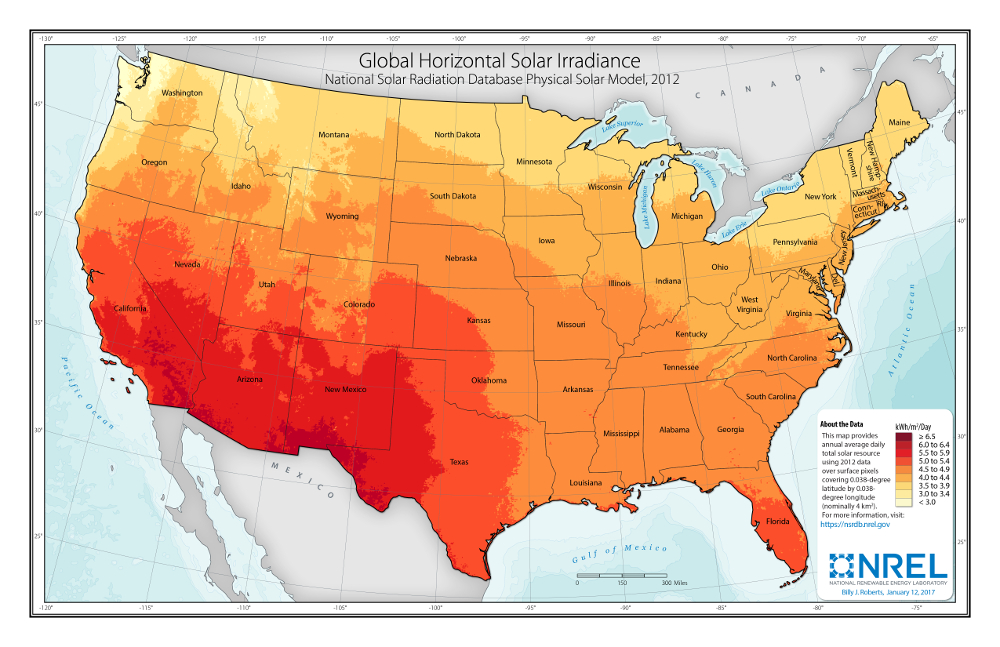
Solar resources across the United States are mostly good to excellent at about 1,000–2,500 kWh)/m2/year. The Southwest is at the top of this range, while only Alaska and part of Washington are at the low end. The range for the contiguous United States is about 1,350–2,500 kWh/m2/year. Nationwide, solar resource levels vary by about a factor of two.
Distributed-scale PV is assumed to be configured as a fixed-axis, roof-mounted system. Compared to utility-scale PV, this reduces both the potential capacity factor and amount of land (roof space) that is available for development. A recent study of rooftop PV technical potential (Gagnon et al. 2016) estimated that as much as 731 GW (926 TWh/yr) of potential exists for small buildings (< 5,000 m2 footprint) and 386 GW (506 TWh/yr) for medium (5,000–25,000 m2) and large buildings (>25,000 m2).
Renewable energy technical potential, as defined by Lopez et al. (2012), represents the achievable energy generation of a particular technology given system performance, topographic limitations, and environmental and land-use constraints. The primary benefit of assessing technical potential is that it establishes an upper-boundary estimate of development potential. It is important to understand that there are multiple types of potential-resource, technical, economic, and market (Lopez et al. 2012; NREL, "Renewable Energy Technical Potential").
Base Year and Projections Overview
The Base Year estimates rely on modeled CAPEX and O&M estimates benchmarked with industry and historical data. Capacity factor is estimated based on hours of sunlight at latitude for all geographic locations in the United States. Capacity factor is estimated based on hours of sunlight at latitude for three representative geographic locations in the United States.
Future year projections are derived from analysis of published projections of PV CAPEX and bottom-up engineering analysis of O&M costs. Three different projections were developed for scenario modeling as bounding levels:
- High cost: no change in CAPEX, O&M, or capacity factor from 2016 to 2050; consistent across all renewable energy technologies in the ATB
- Mid cost: based on the median of literature projections of future CAPEX; O&M technology pathway analysis
- Low cost: based on low bound of literature projections of future CAPEX; O&M technology pathway analysis.
CAPital EXpenditures (CAPEX): Historical Trends, Current Estimates, and Future Projections
Capital expenditures (CAPEX) are expenditures required to achieve commercial operation in a given year. These expenditures include the hardware, the balance of system (e.g., site preparation, installation, and electrical infrastructure), and financial costs (e.g., development costs, onsite electrical equipment, and interest during construction) and are detailed in CAPEX Definition. In the ATB, CAPEX reflects typical plants and does not include differences in regional costs associated with labor or materials. The range of CAPEX demonstrates variation with resource in the contiguous United States.
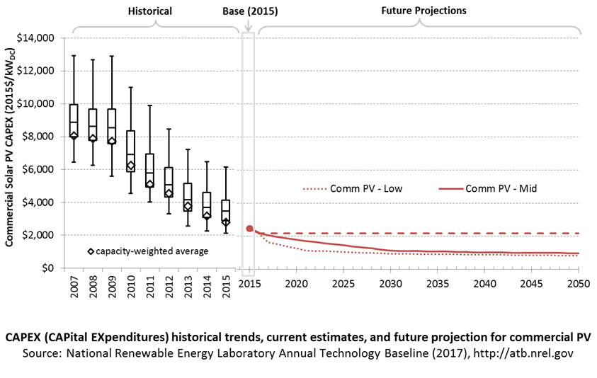
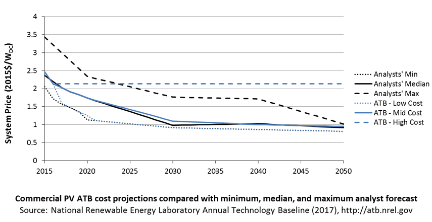
The following figure shows the Base Year estimate and future year projections for CAPEX costs. Three cost reduction scenarios are represented: High, Mid, and Low. Historical data from commercial PV installed in the United States are shown for comparison to the ATB Base Year estimates. The estimate for a given year represents CAPEX of a new plant that reaches commercial operation in that year.
Recent Trends
Reported historical commercial-scale PV installation CAPEX (Barbose and Dargouth 2016) is shown in box-and-whiskers format for comparison to the ATB current CAPEX estimates and future projections. The data in Barbose and Dargouth (2016) represent 85% of all U.S. residential and commercial PV capacity installed through 2015 and 82% of capacity installed in 2015.
PV pricing and capacities are quoted in kWDC (i.e., module rated capacity) unlike other generation technologies, which are quoted in kWAC. For PV, this would correspond to the combined rated capacity of all inverters. This is done because kWDC is the unit that the majority of the PV industry uses. Although costs are reported in kWDC, the total CAPEX includes the cost of the inverter, which has a capacity measured in kWAC.
CAPEX estimates for 2015 reflect continued rapid decline in pricing supported by analysis of recent system pricing for projects that became operational in 2015 (Feldman et al. 2016).
The range in CAPEX estimates reflects the heterogeneous composition of the commercial PV market in the United States.
Base Year Estimates
For illustration in the ATB, a representative commercial-scale PV installation is shown. Although the PV technologies vary, typical installation costs are represented with a single estimate because the CAPEX does not vary with solar resource.
Although the technology market share may shift over time with new developments, the typical installation cost is represented with the projections above.
A system price of $2.47/WDC in 2015 represents the median reported price of a utility-scale PV system installed in 2015 reported in Tracking the Sun IX (Barbose and Dargouth 2016) and adjusted to remove regional cost multipliers based on geographic location of projects installed in 2015. The $2.18/WDC in 2016 is based on bottom-up benchmark analysis reported in U.S. Solar Photovoltaic System Cost Benchmark Q1 2016 (adjusted for inflation) (Fu et al. 2016). These figures are in line with other estimated system prices reported in Feldman et al. (2016).
The Base Year CAPEX estimates should tend toward the low end of observed cost because no regional impacts are included. These effects are represented in the historical market data.
Future Year Projections
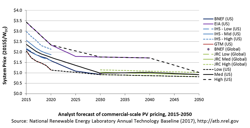
Projections of future commercial PV installation CAPEX are based on 10 system price projections from 5 separate institutions. We adjusted the "min," "median," and "max" analyst forecasts in a few different ways. All 2015 pricing is based on the 20th percentile, median, and 80th percentile historically reported commercial PV prices reported in Tracking the Sun IX (Barbose and Dargouth 2016). All 2016 pricing is based on the bottom-up benchmark analysis reported in U.S. Solar Photovoltaic System Cost Benchmark Q1 2016 (adjusted for inflation) (Fu et al. 2016). These figures are in line with other estimated system prices reported in Feldman et al. (2016).
We adjusted the Mid and Low projections for 2017–2050 to remove distortions caused by the combination of forecasts with different time horizons and based on internal judgment of price trends. The high projection case is kept constant at the 2016 CAPEX value, assuming no improvements beyond 2016.
A detailed description of the methodology for developing Future Year Projections is found in Projections Methodology.
Technology innovations that could impact future O&M costs are summarized in LCOE Projections.
CAPEX Definition
Capital expenditures (CAPEX) are expenditures required to achieve commercial operation in a given year. For commercial PV, this is modeled for a host-owned business model only with access to debt.
For the ATB - and based on EIA (2016a) and the NREL Solar PV Cost Model (Fu et al. 2016) - the distributed solar PV plant envelope is defined to include:
- Hardware
- Module supply
- Power electronics
- Racking
- Foundation
- AC and DC materials and installation
- Balance of system (BOS)
- Site and/or roof preparation
- Permitting, inspection, and interconnection costs
- Project indirect costs, including costs related to engineering, distributable labor and materials, construction management start up and commissioning, and contractor overhead costs, fees, and profit.
- Financial costs
- Owner's costs, such as development costs, legal fees, insurance costs.
- Depreciation and interest on debt (ConFinFactor).
CAPEX can be determined for a plant in a specific geographic location as follows:
CAPEX = ConFinFactor*(OCC*CapRegMult+GCC).
(See the Financial Definitions tab in the ATB data spreadsheet.)
Regional cost variations are not included in the ATB (CapRegMult = 1). Because distributed PV plants are located directly at the end use, there are no grid connection costs (GCC = 0). In the ATB, the input value is overnight capital cost (OCC) and details to calculate interest during construction (ConFinFactor).
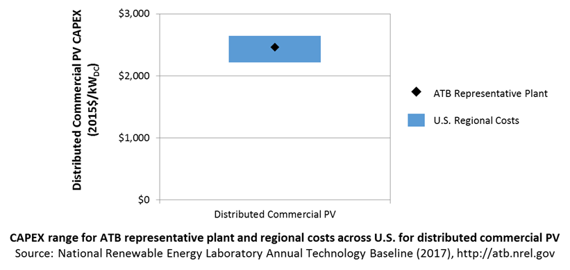
In the ATB, CAPEX represents a typical distributed residential/commercial PV plant and does not vary with resource. Regional cost effects associated with labor rates, material costs, and other regional effects as defined by EIA (2016a) expand the range of CAPEX. Unique land-based spur line costs based on distance and transmission line costs are not estimated. The following figure illustrates the ATB representative plant relative to the range of CAPEX including regional costs across the contiguous United States. The ATB representative plants are associated with a regional multiplier of 1.0.
Standard Scenarios Model Results
ATB CAPEX, O&M, and capacity factor assumptions for the Base Year and future projections through 2050 for High, Mid, and Low projections are used to develop the NREL Standard Scenarios using the ReEDS model. See ATB and Standard Scenarios.
CAPEX in the ATB does not represent regional variants (CapRegMult) associated with labor rates, material costs, etc., but dGen does include state-level cost multipliers (EIA 2016a).
Operation and Maintenance (O&M) Costs
Operations and maintenance (O&M) costs represent the annual expenditures required to operate and maintain a solar PV plant over its technical lifetime of 30 years (the distinction between economic life and technical life is described here), including:
- Insurance, property taxes, site security, legal and administrative fees, and other fixed costs
- Present value, annualized large component replacement costs over technical life (e.g., inverters at 15 years)
- Scheduled and unscheduled maintenance of solar PV plants, transformers, etc. over the technical lifetime of the plant (e.g., general maintenance, including cleaning and vegetation removal).
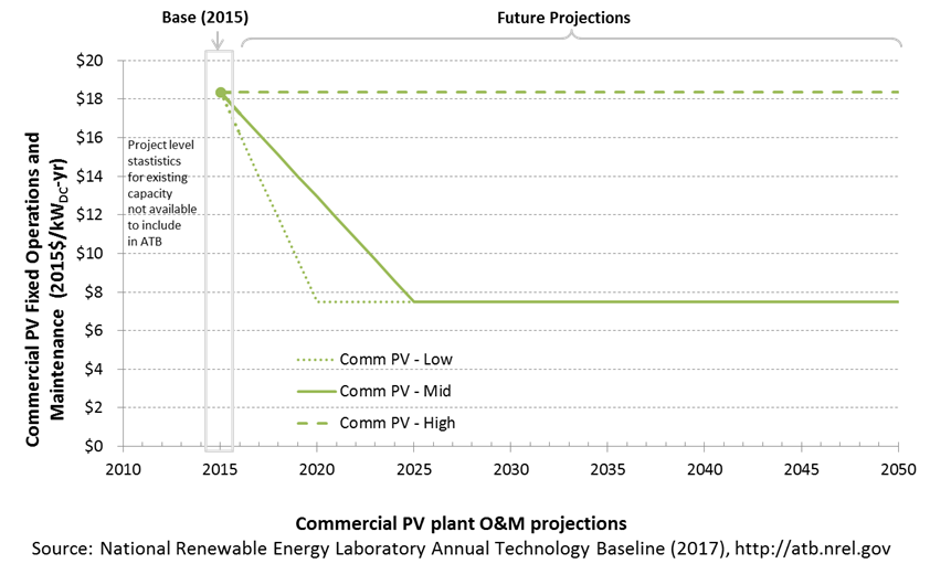
The following figure shows the Base Year estimate and future year projections for fixed O&M (FOM) costs. Three cost reduction scenarios are represented. The estimate for a given year represents annual average FOM costs expected over the technical lifetime of a new plant that reaches commercial operation in that year.
Base Year Estimates
FOM is assumed to be $18/kWDC-yr based on Woodhouse et al. (2016). This number is reasonably consistent with the 2013 "empirical O&M costs" reported in Bolinger and Weaver (2014), which indicates O&M costs ranging from $15/kWAC/yr to $25/kWAC/yr for fixed-tilt PV systems (this range would be lower if reported in $kWDC/yr). A wide range in reported prices exists in the market, in part depending on what maintenance practices exist for a particular system. These cost categories include asset management (including compliance and reporting for incentive payments), different insurance products, site security, cleaning, vegetation removal, and failure of components. Not all these practices are performed for each system; additionally, some factors are dependent on the quality of the parts and construction. NREL analysts estimate O&M costs can range between $0 and $40/kWDC-yr.
Future Year Projections
Future FOM is assumed to decline to $7.5/kWDC-yr by 2020 in the Low cost case and by 2025 in the Mid cost case.
There is currently great market variation in what individual companies perform for O&M.
A detailed description of the methodology for developing Future Year Projections is found in Projections Methodology.
Technology innovations that could impact future CAPEX costs are summarized in LCOE Projections.
Capacity Factor: Expected Annual Average Energy Production Over Lifetime
The capacity factor represents the expected annual average energy production divided by the annual energy production, assuming the plant operates at rated capacity for every hour of the year. It is intended to represent a long-term average over the technical lifetime of the plant (the distinction between economic life and technical life is described here). It does not represent interannual variation in energy production. Future year estimates represent the estimated annual average capacity factor over the technical lifetime of a new plant installed in a given year.
PV system capacity is not directly comparable to other technologies' capacity factors. Other technologies' capacity factors are represented in exclusively AC units (see Solar PV AC-DC Translation). However, because PV pricing in this ATB documentation is represented in $/WDC, PV system capacity is a DC rating. Because each technology uses consistent capacity ratings, the LCOEs are comparable.
The capacity factor is influenced by the hourly solar profile, technology (e.g., thin-film versus crystalline silicon), axis type (e.g., none, one, or two), expected downtime, and inverter losses to transform from DC to AC power. The DC-AC ratio is a design choice that influences the capacity factor. For the ATB, commercial PV systems are modeled for a 300-kWDC fixed-tilt (5°), roof-mounted system. PV plant capacity factor incorporates an assumed degradation rate of 0.5%/year (Jordan and Kurtz 2013) in the annual average calculation.
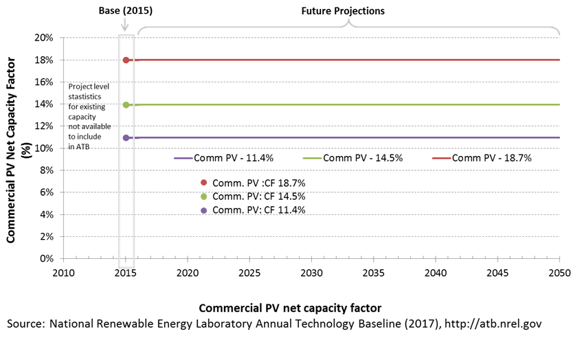
The following figure shows a range of capacity factors based on variation in the solar resource in the contiguous United States. The range of the Base Year estimates illustrate the effect of locating a residential PV plant in locations with solar irradiance similar to Seattle, Washington, Kansas City, Missouri, or Daggett, California (estimated first-year operation capacity factors of 11.4%, 14.5%, and 18.7% respectively). Future projections for High, Mid, and Low cost scenarios are unchanged from the Base Year. Technology improvements are focused on CAPEX and O&M cost elements.
Base Year Estimates
For illustration in the ATB, a range of capacity factors is associated with solar irradiance diversity and the range of latitude for three resource locations in the contiguous United States:
- Low: Seattle, Washington
- Mid: Kansas City, Missouri
- High: Daggett, California
First-year operation capacity factors as modeled range from 11.4% to 18.7%, though these depend significantly on geography and system configuration (e.g., fixed-tilt versus single-axis tracking).
Over time, PV installation output is reduced due to degradation in module quality. This degradation is accounted in ATB estimates of capacity factor over the 20-year economic life of the plant (the distinction between economic life and technical life is described here). The adjusted average capacity factor values in the ATB are 11%, 14%, and 18%.
Future Year Projections
Projections of capacity factor for installations installed in future years are unchanged from the Base Year. Solar PV installations have very little downtime, inverter efficiency is already optimized, and improvements in panel density are expected to result in smaller footprints or lower CAPEX, not necessarily increased capacity factor. That said, there is potential for future increases in capacity factor through technological improvements such as less panel reflectivity, lower degradations rates and improved performance in low-light conditions.
Standard Scenarios Model Results
ATB CAPEX, O&M, and capacity factor assumptions for the Base Year and future projections through 2050 for High, Mid, and Low projections are used to develop the NREL Standard Scenarios using the ReEDS model. See ATB and Standard Scenarios.
dGen does not endogenously consider curtailment from surplus renewable energy generation, though this is a feature of the linked ReEDS-dGen model (Cole et al. 2016), where balancing area-level marginal curtailments can be applied to DPV generation as determined by scenario constraints.
Plant Cost and Performance Projections Methodology
Currently, CAPEX - not LCOE - is the most common metric for PV cost. Due to differing assumptions in long-term incentives, system location and production characteristics, and cost of capital, LCOE can be confusing and often incomparable between differing estimates. While CAPEX also has many assumptions and interpretations, it involves fewer variables to manage. Therefore, PV projections in the ATB are driven entirely by plant and operational cost improvements.
We created High, Mid and Low CAPEX cases to explore the range of possible outcomes of future PV cost improvements. The High cost case represents no CAPEX improvements made beyond today, the Mid cost case represents current expectations of price reductions in a "business-as-usual" scenario, and the Low cost case represents current expectations of potential cost reductions given improved R&D funding and more aggressive global deployment targets.
While CAPEX is one of the drivers to lower costs, R&D efforts continue to focus on other areas to lower the cost of energy from residential PV. While these are not incorporated in the ATB, they include: longer system lifetime, improved performance and reliability, and lower cost of capital.
Projections of future commercial PV installation CAPEX are based on 10 system price projections from 5 separate institutions. Projections included short-term U.S. price forecasts made in the past six months and long-term global and U.S. price forecasts made in the past primarily provided by market analysis firms with expertise in the PV industry, through a subscription service with NREL. The long-term forecasts primarily represent the collection of publicly available, unique forecasts with either a long-term perspective of solar trends or through capacity expansion models with assumed learning by doing.
- Short-term forecast institutions: Bloomberg New Energy Finance, GTM Research, IHS Technology, U.S. Energy Information Administration
- Long-term forecast institutions: Bloomberg New Energy Finance, European Commission's Joint Research Centre, U.S. Energy Information Administration.
In instances in which literature projections did not include all years, a straight-line change in price was assumed between any two projected values. To generate a High, Mid, and Low cost forecast we took the "min," "median," and "max" of the data sets; however, we only included short-term U.S. forecasts until 2030 as they focus on near-term pricing trends within the industry. Starting in 2030, we include long-term global and U.S. forecasts in the data set, as they focus more on long-term trends within the industry. It is also assumed after 2025 U.S. prices will be on par with global averages; the U.S. federal tax credit for solar assets reverts down to 10% for all projects placed in service after 2023, which has the potential to lower upfront financing costs and remove any distortions in reported pricing, compared to other global markets. Additionally, a larger portion of the United States will have a more mature PV market, which should result in a narrower price range. Changes in price for the High, Mid, and Low cost forecast between 2020 and 2030 are interpolated on a straight-line basis.
We adjusted the "min," "median," and "max" analyst forecasts in a few different ways. All 2015 pricing is based on the 20th percentile, median, and 80th percentile historically reported commercial PV price reported in Tracking the Sun IX (Barbose and Dargouth 2016). All 2016 pricing is based on the bottom-up benchmark analysis reported in U.S. Solar Photovoltaic System Cost Benchmark Q1 2016 (adjusted for inflation) (Fu et al. 2016). These figures are in line with other estimated system prices reported in Feldman et al. (2016).
We adjusted the Mid and Low cost projections for 2017-2050 to remove distortions caused by the combination of forecasts with different time horizons and based on internal judgment of price trends. The High cost projection case is kept constant at the 2016 CAPEX value, assuming no improvements beyond 2016.
All prices quoted in WAC are converted to WDC (1 WAC=1.2 WDC).
Future FOM is assumed to decline to $7.5/kWDC-yr by 2020 in the Low case and by 2025 in the Mid case through improvements in system operation and more durable, better performing capital equipment (Woodhouse et al. 2016).
Capacity factors are assumed to not increase over time. All PV system efficiency improvements are assumed to result in capital cost reductions rather than capacity factor improvements.
Levelized Cost of Energy (LCOE) Projections
Levelized cost of energy (LCOE) is a simple metric that combines the primary technology cost and performance parameters, CAPEX, O&M, and capacity factor. It is included in the ATB for illustrative purposes. The focus of the ATB is to define the primary cost and performance parameters for use in electric sector modeling or other analysis where more sophisticated comparisons among technologies are made. LCOE captures the energy component of electric system planning and operation, but the electric system also requires capacity and flexibility services to operate reliably. Electricity generation technologies have different capabilities to provide such services. For example, wind and PV are primarily energy service providers, while the other electricity generation technologies provide capacity and flexibility services in addition to energy. These capacity and flexibility services are difficult to value and depend strongly on the system in which a new generation plant is introduced. These services are represented in electric sector models such as the ReEDS model and corresponding analysis results such as the Standard Scenarios.
The following three figures illustrate the combined impact of CAPEX, O&M, and capacity factor projections across the range of resources present in the contiguous United States. The Current Market Conditions LCOE demonstrates the range of LCOE based on macroeconomic conditions similar to the present. The Historical Market Conditions LCOE presents the range of LCOE based on macroeconomic conditions consistent with prior ATB editions and Standard Scenarios model results. The Normalized LCOE (all LCOE estimates are normalized with the lowest Base Year LCOE value) emphasizes the effect of resource quality and the relative differences in the three future pathways independent of project finance assumptions. The ATB representative plant characteristics that best align with recently installed or anticipated near-term commercial PV plants are associated with Comm PV: 14.5%. Data for all the resource categories can be found in the ATB data spreadsheet.
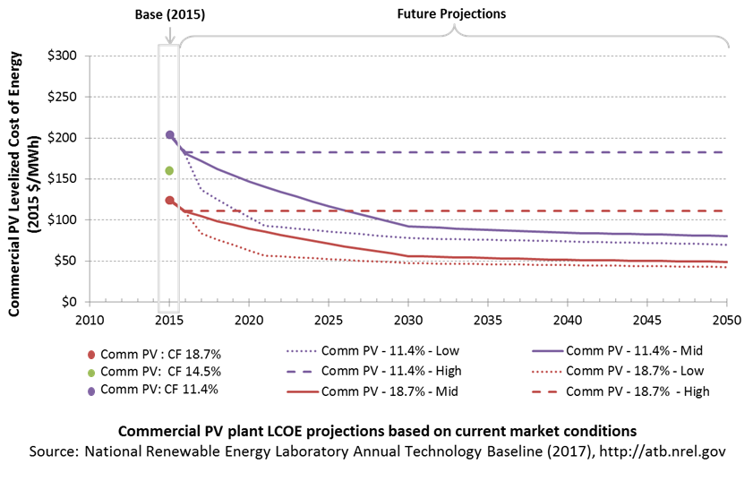
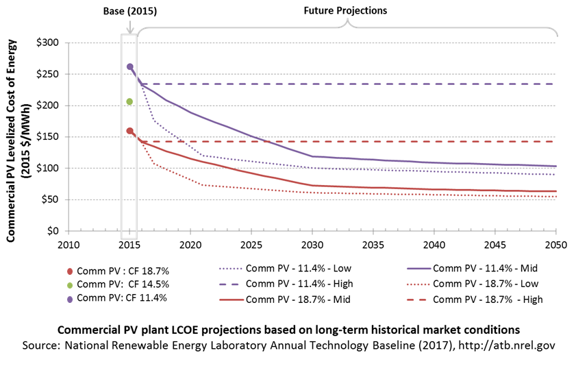
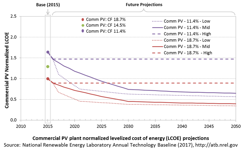
The methodology for representing the CAPEX, O&M, and capacity factor assumptions behind each pathway is discussed in Projections Methodology. The three pathways are generally defined as:
- High = Base Year (or near-term estimates of projects under construction) equivalent through 2050 maintains current relative technology cost differences
- Mid = technology advances through continued industry growth, public and private R&D investments, and market conditions relative to current levels that may be characterized as "likely" or "not surprising"
- Low = Technology advances that may occur with breakthroughs, increased public and private R&D investments, and/or other market conditions that lead to cost and performance levels that may be characterized as the "limit of surprise" but not necessarily the absolute low bound.
To estimate LCOE, assumptions about the cost of capital to finance electricity generation projects are required. For comparison in the ATB, two project finance structures are represented.
- Current Market Conditions: The values of the production tax credit (PTC) and investment tax credit (ITC) are ramping down by 2020, at which time wind and solar projects may be financed with debt fractions similar to other technologies. This scenario reflects debt interest (4.4% nominal, 1.9% real) and return on equity rates (9.5% nominal, 6.8% real) to represent 2017 market conditions (AEO 2017) and a debt fraction of 60% for all electricity generation technologies. An economic life, or period over which the initial capital investment is recovered, of 20 years is assumed for all technologies. These assumptions are one of the project finance options in the ATB spreadsheet.
- Long-Term Historical Market Conditions: Historically, debt interest and return on equity were represented with higher values. This scenario reflects debt interest (8% nominal, 5.4% real) and return on equity rates (13% nominal, 10.2% real) implemented in the ReEDS model and reflected in prior versions of the ATB and Standard Scenarios model results. A debt fraction of 60% for all electricity generation technologies is assumed. An economic life, or period over which the initial capital investment is recovered, of 20 years is assumed for all technologies. These assumptions are one of the project finance options in the ATB spreadsheet.
These parameters are held constant for estimates representing the Base Year through 2050. No incentives such as the PTC or ITC are included. The equations and variables used to estimate LCOE are defined on the equations and variables page. For illustration of the impact of changing financial structures such as WACC and economic life, see Project Finance Impact on LCOE. For LCOE estimates for High, Mid, and Low scenarios for all technologies, see 2017 ATB Cost and Performance Summary.
The LCOE for commercial PV systems is calculated using the same financing parameters as the utility systems. Although we recognize that commercial systems have a wide range of financing options available to them, we represent LCOEs using these utility-based financing calculations in order to allow better comparison against the utility system LCOEs.
In general, the degree of adoption of a range of technology innovations distinguishes the High, Mid and Low cost cases. These projections represent the following trends to reduce CAPEX and FOM.
- Modules
- Increased module efficiencies and increased production-line throughput to decrease CAPEX; overhead costs on a per-kilowatt will go down if efficiency and throughput improvement are realized.
- Reduced wafer thickness or the thickness of thin-film semiconductor layers
- Development of new semiconductor materials
- Development of larger manufacturing facilities in low-cost regions
- Balance of system (BOS)
- Increased module efficiency, reducing the size of the installation
- Development of racking systems that enhance energy production or require less robust engineering
- Integration of racking or mounting components in modules
- Reduction of supply chain complexity and cost
- Creation of standard packages system design
- Improvement of supply chains for BOS components in modules
- Improved power electronics
- Improvement of inverter prices and performance, possibly by integrating micro-inverters
- Decreased installation costs and margins
- Reduction of supply chain margins (e.g., profit and overhead charged by suppliers, manufacturer, distributors, and retailers); this will likely occur naturally as the U.S. PV industry grows and matures.
- Streamlining of installation practices through improved workforce development and training, and developing standardized PV hardware
- Expansion of access to a range of innovative financing approaches and business models
- Development of best practices for permitting interconnection, and PV installation such as subdivision regulations, new construction guidelines, and design requirements.
FOM cost reduction represents optimized O&M strategies, reduced component replacement costs, and lower frequency of component replacement.
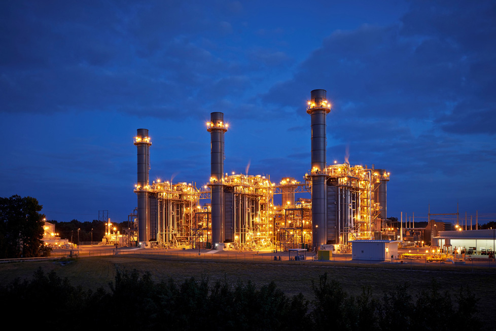
Natural Gas Plants
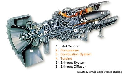
A gas-fired combustion turbine involves:
- An air compressor compresses air and feeds it into the combustion chamber at hundreds of miles per hour.
- In a combustion system, a ring of fuel injectors inject fuel into combustion chambers where it mixes with the air and is combusted. The resulting high-temperature, high-pressure gas stream enters and expands through the turbine.
- A turbine has alternate stationary and rotating airfoil-section blades that are driven by expanding hot combustion gas. The rotating blades drive the compressor and spin a generator to produce electricity.
Simple-cycle gas turbines can achieve 20%-35% energy conversion efficiency depending on the type and design of the system. Aeroderivative turbines are typically more flexible but more expensive than their industrial gas turbine counterparts. Combined-cycle natural gas plants include a heat recovery steam generator that uses the hot exhaust from the combustion turbine to generate steam. That steam can then be used to generate additional electricity using a steam turbine. Combined-cycle natural gas plants typically have efficiencies ranging from 50%-60%, and R&D targets have been set to achieve even higher efficiencies. Combined-cycle plants can be built using a variety of configurations, such as a single combustion turbine and steam turbine connected to a single generator (1x1) or two combustion turbines coupled with one steam turbine (2x1) (DOE "How Gas Turbine Power Plants Work").
Renewable energy technical potential, as defined by Lopez et al. (2012), represents the achievable energy generation of a particular technology given system performance, topographic limitations, and environmental and land-use constraints. Technical resource potential corresponds most closely to fossil reserves, as both can be characterized by the prospect of commercial feasibility and depend strongly on available technology at the time of the resource assessment. Natural gas reserves in the United States are assessed by the United States Geological Survey (USGS, "National Oil and Gas Assessment").
This section focuses on large, utility-scale natural gas plants. Distributed-scale turbines may be included in a future version of the ATB.
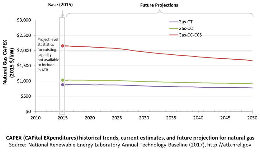
CAPital EXpenditures (CAPEX): Historical Trends, Current Estimates, and Future Projections
Because natural gas plants are well-known and perform close to their optimal performance, the EIA capital expenditures (CAPEX) projections decline at the minimum learning rate for the gas-fired technologies, resulting in incremental improvement over time that progresses slightly more quickly than inflation.
The one exception is natural gas combined cycle (CC) with carbon capture and storage (CCS). The DOE Office of Fossil Energy and the National Energy Technology Laboratory conduct research on reducing the costs and increasing the performance of CCS technology, and costs are expected to decline over time at a higher learning rate than the more mature gas-CT and gas-CC technologies.
Comparison with Other Sources
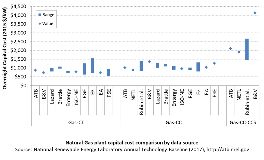
Costs vary due to differences in configuration (e.g., 2x1 versus 1x1), turbine class, and methodology. All costs were converted to the same dollar year.
CAPEX Definition
Capital expenditures (CAPEX) are expenditures required to achieve commercial operation in a given year.
Overnight capital costs are modified from EIA (2017). Capital costs include overnight capital cost plus defined transmission cost, and it removes a material price index.
Fuel costs are taken from EIA (2017). EIA reports two types of gas-CT and gas-CC technologies in the Annual Energy Outlook: advanced (H-class for gas-CC, F-class for gas-CT) and conventional (F-class for gas-CC, LM-6000 for gas-CT). Because we represent a single gas-CT and gas-CC technology in the ATB, the characteristics for the ATB plants are taken to be the average of the advanced and conventional systems as reported by EIA. For example, the OCC for the gas-CC technology in the ATB is the average of the capital cost of the advanced and conventional combined cycle technologies from the EIA's Annual Energy Outlook. Future work aims to improve the representation of the various natural gas technologies in the ATB. The CCS plant configuration includes only the cost of capturing and compressing the CO2. It does not include CO2 delivery and storage.
| Overnight Capital Cost ($/kW) | Construction Financing Factor (ConFinFactor) | CAPEX ($/kW) | |
|---|---|---|---|
| Gas-CT: Conventional combustion turbine | $864 | 1.021 | $882 |
| Gas-CC: Conventional combined cycle | $1,010 | 1.021 | $1,032 |
| Gas-CC-CCS: Combined cycle with carbon capture sequestration | $2,109 | 1.021 | $2,154 |
CAPEX can be determined for a plant in a specific geographic location as follows:
CAPEX = ConFinFactor × (OCC×CapRegMult+GCC).
(See the Financial Definitions tab in the ATB data spreadsheet.)
Regional cost variations and geographically specific grid connection costs are not included in the ATB (CapRegMult=1; GCC=0). In the ATB, the input value is overnight capital cost (OCC) and details to calculate interest during construction (ConFinFactor).
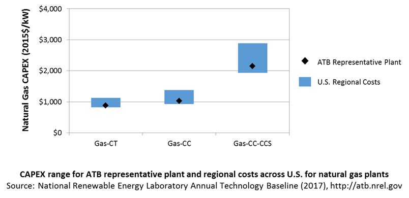
In the ATB, CAPEX represents each type of gas plant with a unique value. Regional cost effects associated with labor rates, material costs, and other regional effects as defined by EIA (2016a) expand the range of CAPEX. Unique land-based spur line costs based on distance and transmission line costs are not estimated. The following figure illustrates the ATB representative plant relative to the range of CAPEX including regional costs across the contiguous United States. The ATB representative plants are associated with a regional multiplier of 1.0.
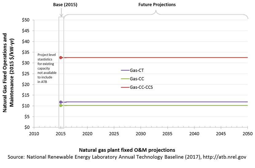
Operation and Maintenance (O&M) Costs
Operations and maintenance (O&M) costs represent the annual expenditures required to operate and maintain a plant over its technical lifetime (the distinction between economic life and technical life is described here), including:
- Insurance, taxes, land lease payments, and other fixed costs
- Present value and annualized large component replacement costs over technical life
- Scheduled and unscheduled maintenance of power plants, transformers, and other components over the technical lifetime of the plant.
Market data for comparison are limited and generally inconsistent in the range of costs covered and the length of the historical record.
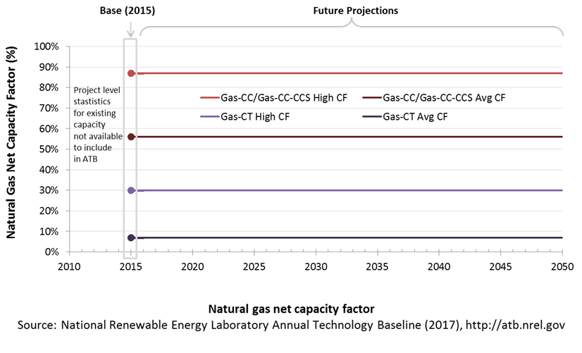
Capacity Factor: Expected Annual Average Energy Production Over Lifetime
The capacity factor represents the assumed annual energy production divided by the total possible annual energy production, assuming the plant operates at rated capacity for every hour of the year. For natural gas plants, the capacity factor is typically lower (and, in the case of combustion turbines, much lower) than their availability factor. Natural gas plants have availability factors approaching 100%.
The capacity factors of dispatchable units is typically a function of the unit's marginal costs and local grid needs (e.g., need for voltage support or limits due to transmission congestion). The average capacity factor is the average fleet-wide capacity factor for these plant types in 2015. The high capacity factor is taken from EIA (2016c, Table 1a) for a new power plant and represents a high bound of operation for a plant of this type.
Gas-CT power plants are less efficient than gas-CC power plants, and they tend to run as intermediate or peaker plants.
Gas-CC with CCS has not yet been built. It is expected to be a baseload unit.
Levelized Cost of Energy (LCOE) Projections
Levelized cost of energy (LCOE) is a simple metric that combines the primary technology cost and performance parameters, CAPEX, O&M, and capacity factor. It is included in the ATB for illustrative purposes. The focus of the ATB is to define the primary cost and performance parameters for use in electric sector modeling or other analysis where more sophisticated comparisons among technologies are made. LCOE captures the energy component of electric system planning and operation, but the electric system also requires capacity and flexibility services to operate reliably. Electricity generation technologies have different capabilities to provide such services. For example, wind and PV are primarily energy service providers, while the other electricity generation technologies provide capacity and flexibility services in addition to energy. These capacity and flexibility services are difficult to value and depend strongly on the system in which a new generation plant is introduced. These services are represented in electric sector models such as the ReEDS model and corresponding analysis results such as the Standard Scenarios.
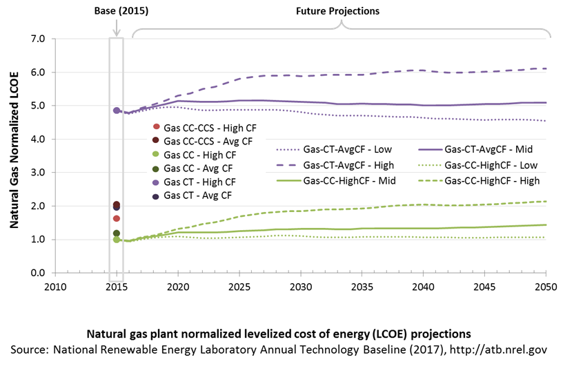
The following three figures illustrate the combined impact of CAPEX, O&M, and capacity factor projections across the range of resources present in the contiguous United States. The Current Market Conditions LCOE demonstrates the range of LCOE based on macroeconomic conditions similar to the present. The Historical Market Conditions LCOE presents the range of LCOE based on macroeconomic conditions consistent with prior ATB editions and Standard Scenarios model results. The Normalized LCOE (all LCOE estimates are normalized with the lowest Base Year LCOE value) emphasizes the relative effect of fuel price and heat rate independent of project finance assumptions. The ATB representative plant characteristics that best align with recently installed or anticipated near-term natural gas plants are associated with Gas-CC-HighCF. Data for all the resource categories can be found in the ATB data spreadsheet.
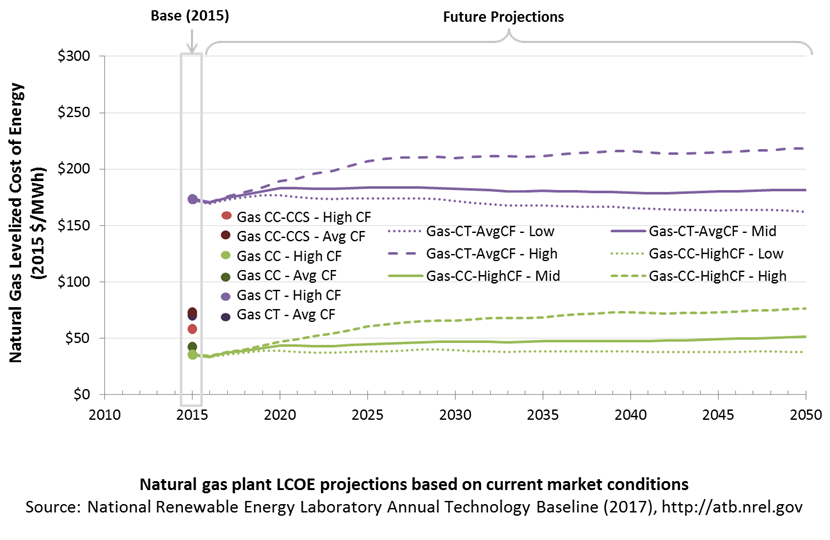
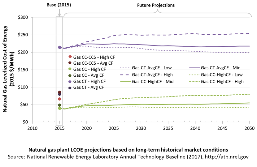
The LCOE of natural gas plants is directly impacted by the price of the natural gas fuel, so we include low, median, and high natural gas price trajectories. The LCOE is also impacted by variations in the heat rate and O&M costs. Because the reference and high natural gas price projections from AEO 2017 are rising over time, the LCOE of new natural gas plants can actually increase over time if the gas prices rise faster than the capital costs decline. For a given year, the LCOE assumes that the fuel prices from that year continue throughout the lifetime of the plant.
These projections do not include any cost of carbon, which would influence the LCOE of fossil units. Also, for CCS plants, the potential revenue from selling the captured carbon is not included (e.g., enhanced oil recovery operation may purchase CO2 from a CCS plant).
Fuel prices are based on the EIA's Annual Energy Outlook 2017 (EIA 2017).
To estimate LCOE, assumptions about the cost of capital to finance electricity generation projects are required. For comparison in the ATB, two project finance structures are represented.
- Current Market Conditions: The values of the production tax credit (PTC) and investment tax credit (ITC) are ramping down by 2020, at which time wind and solar projects may be financed with debt fractions similar to other technologies. This scenario reflects debt interest (4.4% nominal, 1.9% real) and return on equity rates (9.5% nominal, 6.8% real) to represent 2017 market conditions (AEO 2017) and a debt fraction of 60% for all electricity generation technologies. An economic life, or period over which the initial capital investment is recovered, of 20 years is assumed for all technologies. These assumptions are one of the project finance options in the ATB spreadsheet.
- Long-Term Historical Market Conditions: Historically, debt interest and return on equity were represented with higher values. This scenario reflects debt interest (8% nominal, 5.4% real) and return on equity rates (13% nominal, 10.2% real) implemented in the ReEDS model and reflected in prior versions of the ATB and Standard Scenarios model results. A debt fraction of 60% for all electricity generation technologies is assumed. An economic life, or period over which the initial capital investment is recovered, of 20 years is assumed for all technologies. These assumptions are one of the project finance options in the ATB spreadsheet.
These parameters are held constant for estimates representing the Base Year through 2050. No incentives such as the PTC or ITC are included. The equations and variables used to estimate LCOE are defined on the equations and variables page. For illustration of the impact of changing financial structures such as WACC and economic life, see Project Finance Impact on LCOE. For LCOE estimates for High, Mid, and Low scenarios for all technologies, see 2017 ATB Cost and Performance Summary.
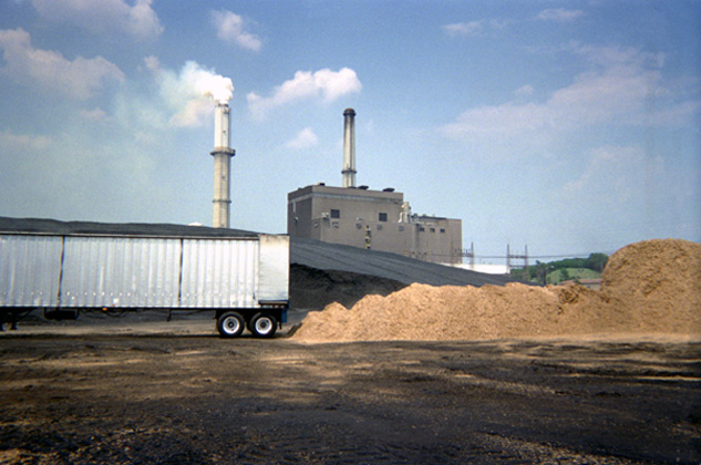
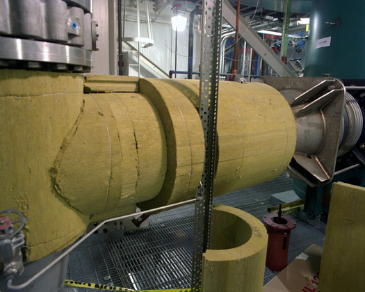
Biopower Plants
In a biopower plant:
- Heat is created: Biomass (sometimes co-fired with coal) is pulverized, mixed with hot air, and burned in suspension.
- Water turns to steam: The heat turns purified water into steam, which is piped to the turbine.
- Steam turns the turbine: The pressure of the steam pushes the turbine blade, turns the shaft in the generator, and creates power.
- Steam is turned back into water: Cool water is drawn into a condenser where the steam turns back into water that can be reused in the plant.
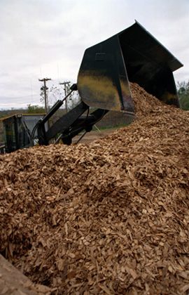
(a biomass gasifier that operates on wood chips)
Renewable energy technical potential, as defined by Lopez et al. (2012), represents the achievable energy generation of a particular technology given system performance, topographic limitations, and environmental and land-use constraints. Technical resource potential for biopower is based on estimated biomass quantities from the Billion Ton Update study (DOE 2011).
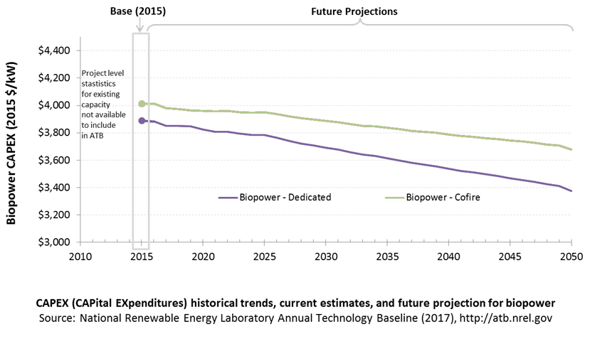
CAPital EXpenditures (CAPEX): Historical Trends, Current Estimates, and Future Projections
Because biopower plants are well-known and perform close to their optimal performance, EIA expects capital expenditures (CAPEX) will incrementally improve over time and slightly more quickly than inflation.
The exception is new biomass cofiring, which is expected to have costs that decline a bit more than existing cofiring project technologies.
CAPEX Definition
Capital expenditures (CAPEX) are expenditures required to achieve commercial operation in a given year.
Overnight capital costs are modified from EIA (2014). Capital costs include overnight capital cost plus defined transmission cost, and it removes a material price index. The overnight capital costs for cofired units are not the cost of upgrading a plant but the total cost of the plant after the upgrade.
Fuel costs are taken from the Billion Ton Update study (DOE 2011).
| Overnight Capital Cost ($/kW) | Construction Financing Factor (ConFinFactor) | CAPEX ($/kW) | |
|---|---|---|---|
| Dedicated: Dedicated biopower plant | $3,737 | 1.041 | $3,889 |
| CofireOld: Pulverized coal with sulfur dioxide (SO2) scrubbers and biomass co-firing | $3,856 | 1.041 | $4,013 |
| CofireNew: Advanced supercritical coal with SO2 and NOx controls and biomass co-firing | $3,856 | 1.041 | $4,013 |
CAPEX can be determined for a plant in a specific geographic location as follows:
CAPEX = ConFinFactor*(OCC*CapRegMult+GCC).
(See the Financial Definitions tab in the ATB data spreadsheet.)
Regional cost variations and geographically specific grid connection costs are not included in the ATB (CapRegMult = 1; GCC = 0). In the ATB, the input value is overnight capital cost (OCC) and details to calculate interest during construction (ConFinFactor).
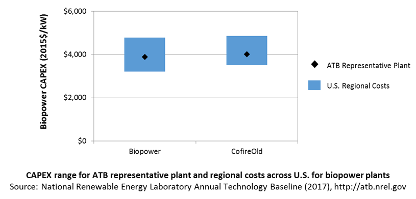
In the ATB, CAPEX represents each type of biopower plant with a unique value. Regional cost effects associated with labor rates, material costs, and other regional effects as defined by EIA (2016a) expand the range of CAPEX. Unique land-based spur line costs based on distance and transmission line costs are not estimated. The following figure illustrates the ATB representative plant relative to the range of CAPEX including regional costs across the contiguous United States. The ATB representative plants are associated with a regional multiplier of 1.0.
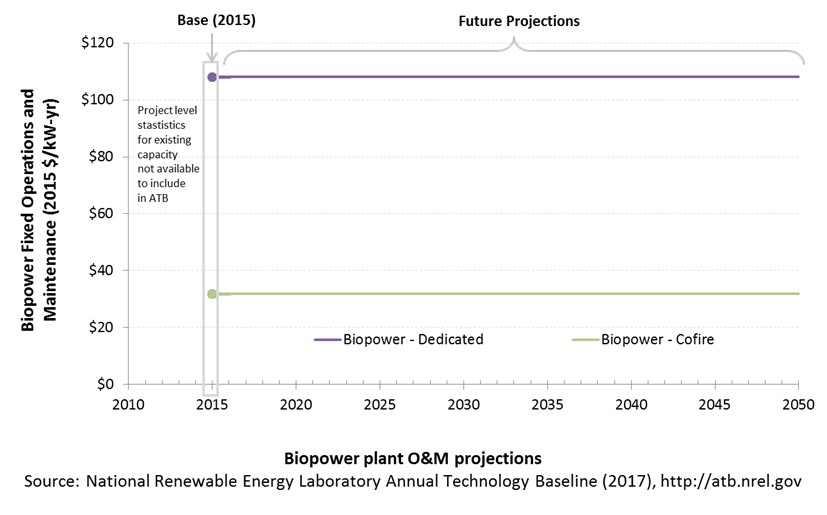
Operation and Maintenance (O&M) Costs
Operations and maintenance (O&M) costs represent the annual expenditures required to operate and maintain a plant over its technical lifetime (the distinction between economic life and technical life is described here), including:
- Insurance, taxes, land lease payments, and other fixed costs
- Present value and annualized large component replacement costs over technical life
- Scheduled and unscheduled maintenance of power plants, transformers, and other components over the technical lifetime of the plant.
Market data for comparison are limited and generally inconsistent in the range of costs covered and the length of the historical record.
Capacity Factor: Expected Annual Average Energy Production Over Lifetime
The capacity factor represents the assumed annual energy production divided by the total possible annual energy production, assuming the plant operates at rated capacity for every hour of the year. For biopower plants, the capacity factors are typically lower than their availability factors. Biopower plant availability factors have a wide range depending on system design, fuel type and availability, and maintenance schedules.
Biopower plants are typically baseload plants with steady capacity factors. For the ATB, the biopower capacity factor is taken as the average capacity factor for biomass plants for 2015, as reported by EIA.
Biopower capacity factors are influenced by technology and feedstock supply, expected downtime, and energy losses.

Levelized Cost of Energy (LCOE) Projections
Levelized cost of energy (LCOE) is a simple metric that combines the primary technology cost and performance parameters, CAPEX, O&M, and capacity factor. It is included in the ATB for illustrative purposes. The focus of the ATB is to define the primary cost and performance parameters for use in electric sector modeling or other analysis where more sophisticated comparisons among technologies are made. LCOE captures the energy component of electric system planning and operation, but the electric system also requires capacity and flexibility services to operate reliably. Electricity generation technologies have different capabilities to provide such services. For example, wind and PV are primarily energy service providers, while the other electricity generation technologies provide capacity and flexibility services in addition to energy. These capacity and flexibility services are difficult to value and depend strongly on the system in which a new generation plant is introduced. These services are represented in electric sector models such as the ReEDS model and corresponding analysis results such as the Standard Scenarios.
The following three figures illustrate the combined impact of CAPEX, O&M, and capacity factor projections across the range of resources present in the contiguous United States. The Current Market Conditions LCOE demonstrates the range of LCOE based on macroeconomic conditions similar to the present. The Historical Market Conditions LCOE presents the range of LCOE based on macroeconomic conditions consistent with prior ATB editions and Standard Scenarios model results. The Normalized LCOE (all LCOE estimates are normalized with the lowest Base Year LCOE value) emphasizes the relative effect of fuel price and heat rate independent of project finance assumptions. Data for all the resource categories can be found in the ATB data spreadsheet.
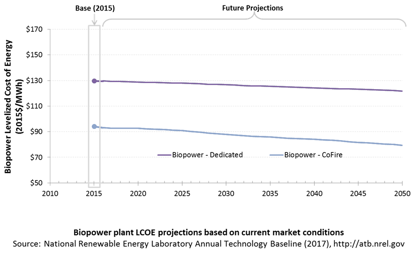
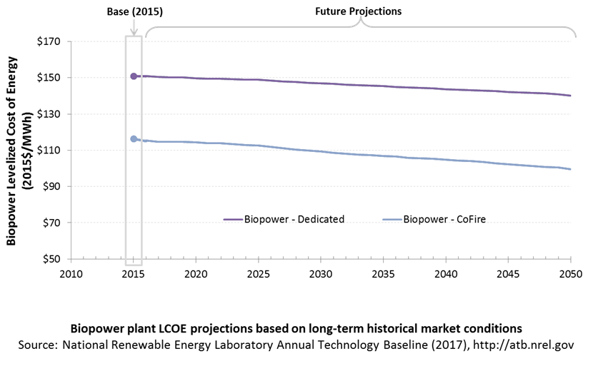
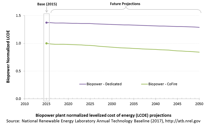
The LCOE of biopower plants is directly impacted by the differences in CAPEX (installed capacity costs) as well as by heat rate differences. For a given year, the LCOE assumes that the fuel prices from that year continue throughout the lifetime of the plant.
Regional variations will ultimately impact biomass feedstock costs, but these are not included in the ATB.
The projections do not include any cost of carbon.
Fuel prices are based on the EIA's Annual Energy Outlook 2017 (EIA 2017).
To estimate LCOE, assumptions about the cost of capital to finance electricity generation projects are required. For comparison in the ATB, two project finance structures are represented.
- Current Market Conditions: The values of the production tax credit (PTC) and investment tax credit (ITC) are ramping down by 2020, at which time wind and solar projects may be financed with debt fractions similar to other technologies. This scenario reflects debt interest (4.4% nominal, 1.9% real) and return on equity rates (9.5% nominal, 6.8% real) to represent 2017 market conditions (AEO 2017) and a debt fraction of 60% for all electricity generation technologies. An economic life, or period over which the initial capital investment is recovered, of 20 years is assumed for all technologies. These assumptions are one of the project finance options in the ATB spreadsheet.
- Long-Term Historical Market Conditions: Historically, debt interest and return on equity were represented with higher values. This scenario reflects debt interest (8% nominal, 5.4% real) and return on equity rates (13% nominal, 10.2% real) implemented in the ReEDS model and reflected in prior versions of the ATB and Standard Scenarios model results. A debt fraction of 60% for all electricity generation technologies is assumed. An economic life, or period over which the initial capital investment is recovered, of 20 years is assumed for all technologies. These assumptions are one of the project finance options in the ATB spreadsheet.
These parameters are held constant for estimates representing the Base Year through 2050. No incentives such as the PTC or ITC are included. The equations and variables used to estimate LCOE are defined on the equations and variables page. For illustration of the impact of changing financial structures such as WACC and economic life, see Project Finance Impact on LCOE. For LCOE estimates for High, Mid, and Low scenarios for all technologies, see 2017 ATB Cost and Performance Summary.
References
B&V (Black & Veatch). 2012. Cost and Performance Data for Power Generation Technologies. Black & Veatch Corporation. February 2012. http://bv.com/docs/reports-studies/nrel-cost-report.pdf.
Barbose, Galen, and Naïm Dargouth. 2016. Tracking the Sun IX: The Installed Price of Residential and Non-Residential Photovoltaic Systems in the United States. Berkeley, CA: Lawrence Berkeley National Laboratory. LBNL-1006036. August 2016. https://emp.lbl.gov/sites/default/files/tracking_the_sun_ix_report.pdf.
Bolinger, Mark, and Samantha Weaver. 2014. Utility Scale Solar 2013: An Empirical Analysis of Project Cost, Performance, and Pricing Trends in the United States. Berkeley, CA: Lawrence Berkeley National Laboratory. September 2014. https://emp.lbl.gov/sites/default/files/lbnl_utility-scale_solar_2013_report.pdf.
Brattle Group (Samuel A. Newell, J. Michael Hagerty, Kathleen Spees, Johannes P. Pfeifenberger, Quincy Liao, Christopher D. Ungate, and John Wroble). 2014. Cost of New Entry Estimates for Combustion Turbine and Combined Cycle Plants in PJM. The Brattle Group. http://www.brattle.com/system/publications/pdfs/000/005/010/original/Cost_of_New_Entry_Estimates_for_Combustion_Turbine_and_Combined_Cycle_Plants_in_PJM.pdf.
Cole, Wesley, Haley Lewis, Ben Sigrin, and Robert Margolis. 2016. 'Interactions of Rooftop PV Deployment with the Capacity Expansion of the Bulk Power System.' Applied Energy 168 (April):473–481. doi:10.1016/j.apenergy.2016.02.004.
DOE (U.S. Department of Energy). 2011. U.S. Billion-Ton Update: Biomass Supply for a Bioenergy and Bioproducts Industry. Perlack, R.D., and B.J. Stokes, eds. Oak Ridge, TN: Oak Ridge National Laboratory. ORNL/TM-2011/224. August 2011. https://www.osti.gov/scitech/biblio/1023318.
E3 (Energy and Environmental Economics). 2014. Capital Cost Review of Power Generation Technologies: Recommendations for WECC's 10- and 20-Year Studies. Prepared for the Western Electric Coordinating Council. https://www.wecc.biz/Reliability/2014_TEPPC_Generation_CapCost_Report_E3.pdf.
EIA (U.S. Energy Information Administration). 2014. Annual Energy Outlook 2014 with Projections to 2040. Washington, D.C.: U.S. Department of Energy. DOE/EIA-0383(2014). April 2014. http://www.eia.gov/forecasts/aeo/pdf/0383(2014).pdf.
EIA (U.S. Energy Information Administration). 2015. Annual Energy Outlook with Projections to 2040. Washington, D.C.: U.S. Department of Energy. DOE/EIA-0383(2015). April 2015. http://www.eia.gov/outlooks/aeo/pdf/0383(2015).pdf.
EIA (U.S. Energy Information Administration). 2016a. Capital Cost Estimates for Utility Scale Electricity Generating Plants. Washington, D.C.: U.S. Department of Energy. November 2016. https://www.eia.gov/analysis/studies/powerplants/capitalcost/pdf/capcost_assumption.pdf.
EIA (U.S. Energy Information Administration). 2016c. Levelized Cost and Levelized Avoided Cost of New Generation Resources in the Annual Energy Outlook 2017. Washington, D.C.: U.S. Department of Energy. April 2017. https://www.eia.gov/outlooks/aeo/pdf/electricity_generation.pdf.
EIA (U.S. Energy Information Administration). 2017. Annual Energy Outlook 2017 with Projections to 2050. Washington, D.C.: U.S. Department of Energy. January 5, 2017. http://www.eia.gov/outlooks/aeo/pdf/0383(2017).pdf.
Entergy. 2015. Entergy Arkansas, Inc.: 2015 Integrated Resource Plan. July 15, 2015. http://entergy-arkansas.com/content/transition_plan/IRP_Materials_Compiled.pdf.
Feldman, David, Robert Margolis, Paul Denholm, and Joseph Stekli. 2016. Exploring the Potential Competitiveness of Utility-Scale Photovoltaics plus Batteries with Concentrating Solar Power, 2015–2030. Golden, CO: National Renewable Energy Laboratory. NREL/TP-6A20-66592. August 2016. http://www.nrel.gov/docs/fy16osti/66592.pdf.
Fu, Ran, Donald Chung, Travis Lowder, David Feldman, Kristen Ardani, and Robert Margolis. 2016. U.S. Photovoltaic (PV) Prices and Cost Breakdowns: Q1 2016 Benchmarks for Residential, Commercial, and Utility-Scale Systems. Golden, CO: National Renewable Energy Laboratory. NREL/PR-6A20-67142. September 2016. http://www.nrel.gov/docs/fy16osti/67142.pdf.
Gagnon, Pieter, Robert Margolis, Jennifer Melius, Caleb Phillips, and Ryan Elmore. 2016. Rooftop Solar Photovoltaic Technical Potential in the United States: A Detailed Assessment. Golden, CO: National Renewable Energy Laboratory. NREL/TP-6A20-65298. https://www.nrel.gov/docs/fy16osti/65298.pdf.
Jordan, Dirk C., and Sarah R. Kurtz. 2013. Photovoltaic Degradation Rates: An Analytical Review. Golden, CO: National Renewable Energy Laboratory. NREL/JA-5200-51664. http://onlinelibrary.wiley.com/doi/10.1002/pip.1182/full.
Lazard. 2016. Levelized Cost of Energy Analysis-Version 10.0. December 2016. New York: Lazard. https://www.lazard.com/media/438038/levelized-cost-of-energy-v100.pdf.
Lopez, Anthony, Billy Roberts, Donna Heimiller, Nate Blair, and Gian Porro. 2012. U.S. Renewable Energy Technical Potentials: A GIS-Based Analysis. National Renewable Energy Laboratory. NREL/TP-6A20-51946. http://www.nrel.gov/docs/fy12osti/51946.pdf.
NETL (National Energy Technology Laboratory: Tim Fout, Alexander Zoelle, Dale Keairns, Marc Turner, Mark Woods, Norma Kuehn, Vasant Shah, Vincent Chou, Lora Pinkerton). 2015. Fossil Energy Plants: Volume 1a: Bituminous Coal (PC) and Natural Gas to Electricity, Revision 3. DOE/NETL-2015/1723. http://www.netl.doe.gov/File%20Library/Research/Energy%20Analysis/Publications/Rev3Vol1aPC_NGCC_final.pdf.
PGE (Portland General Electric). 2015. Integrated Resource Plan 2016. July 16, 2015. https://www.portlandgeneral.com/-/media/public/our-company/energy-strategy/documents/2015-07-16-public-meeting.pdf.
PSE (Puget Sound Energy). 2016. 2017 IRP Supply-Side Resource Advisory Committee: Thermal. July 25, 2016. https://pse.com/aboutpse/EnergySupply/Documents/IRP_07-25-2016_Presentations.pdf.
Rubin, Edward S., Inês M.L. Azevedo, Paulina Jaramillo, and Sonia Yeh. 2015. 'A Review of Learning Rates for Electricity Supply Technologies.' Energy Policy 86 (November 2015): 198–218. http://www.sciencedirect.com/science/article/pii/S0301421515002293.
Woodhouse, Michael, Rebecca Jones-Albertus, David Feldman, Ran Fu, Kelsey Horowitz, Donald Chung, Dirk Jordan, and Sarah Kurtz. 2016. On the Path to SunShot: The Role of Advancements in Solar Photovoltaic Efficiency, Reliability, and Costs. Golden, CO: National Renewable Energy Laboratory. NREL/TP-6A20-65464. May 2016. http://www.nrel.gov/docs/fy16osti/65872.pdf.