Annual Technology Baseline 2018
National Renewable Energy Laboratory
Recommended Citation:
NREL (National Renewable Energy Laboratory). 2018. 2018 Annual Technology Baseline. Golden, CO: National Renewable Energy Laboratory. http://atb.nrel.gov/.
Please consult Guidelines for Using ATB Data:
https://atb.nrel.gov/electricity/user-guidance.html
2018 ATB
For each electricity generation technology in the ATB, this website provides:
- Capital expenditures (CAPEX): the definition of CAPEX used in the ATB and the historical trends, current estimates, and future projections of CAPEX used in the ATB
- Operations and maintenance (O&M) costs: the definition of O&M and the current estimates and future projections of O&M used in the ATB
- Capacity factor (CF): the definition of CF and the historical trends, current estimates, and future projections of CF used in the ATB
- Future cost and performance methods: an outline of the methodology used to make the projections of future cost and performance in the ATB for Constant, Mid, and Low technology cost cases
- Levelized cost of energy (LCOE): metric that combines CAPEX, O&M, CF, and projections for Constant, Mid, and Low technology cost cases for illustration of the combined effect of the primary cost and performance components and discussion of technology advances that yield future projections
- Financing Assumptions: Where applicable, development of technology-specific interest rate on debt, return on equity, and debt-to-equity ratios, and their impact on LCOE are documented in each technology section, and summarized here.
Electricity generation technologies are selected on the left side of the screen, and the topics highlighted above can be selected using the drop-down menu at the top-right of the screen.
Guidelines for using and interpreting ATB content and comparisons to other literature are provided. LCOE accounts for many variables important to determining the competitiveness of a building and operating a specific technology (e.g., upfront capital costs, capacity factor, and cost of financing); however, it does not necessarily demonstrate which technology in a given place and time would provide the lowest cost option for the electricity grid. This analysis is performed using electric sector models such as the Regional Energy Deployment Systems (ReEDS) model and corresponding analysis results such as the NREL Standard Scenarios.
The NREL Standard Scenarios, a companion product to the ATB, provides a suite of electric sector scenarios and associated assumptions-including technology cost and performance assumptions from the ATB.
ATB data sources and references are also provided for each technology. All dollar values are presented in 2016 U.S. dollars, unless noted otherwise.
Additional information about the 2018 ATB - available via links in the ATB website footer below - includes:
Land-Based Wind
Representative Technology
Most land-based wind plants in the United States range in capacity from 50 MW to 100 MW (Wiser and Bolinger (2017)). Wind turbines installed in the United States in 2016 were, on average, 2.2-MW turbines with rotor diameters of 108 m and hub heights of 84 m (Wiser and Bolinger (2017)).
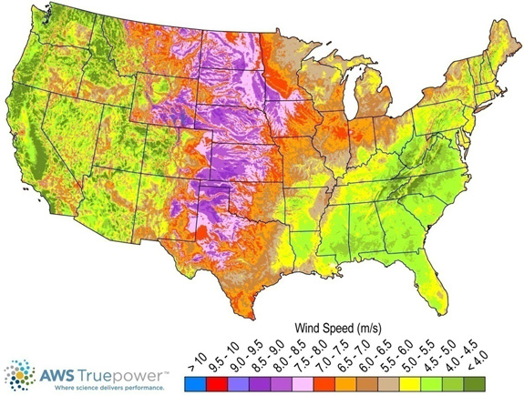
Resource Potential
Wind resource is prevalent throughout the United States but is concentrated in the central states. Total land-based wind technical potential exceeds 10,000 GW (almost tenfold current total U.S. electricity generation capacity), which would use the wind resource on 3.5 million km2 of land area but would disrupt or exclude other uses from a fraction of that area. This technical potential does not include standard exclusions-lands such as federally protected areas, urban areas, and water. Resource potential has been expanded from approximately 6,000 GW (DOE (2015)) by including locations with lower wind speeds to provide more comprehensive coverage of U.S. land areas where future technology may improve economic potential).
Renewable energy technical potential, as defined by Lopez et al. 2012, represents the achievable energy generation of a particular technology given system performance, topographic limitations and environmental and land-use constraints. The primary benefit of assessing technical potential is that it establishes an upper-boundary estimate of development potential. It is important to understand that there are multiple types of potential-resource, technical, economic, and market (Lopez et al. 2012; NREL, "Renewable Energy Technical Potential ").
The resource potential is calculated by using over 130,000 distinct areas for wind plant deployment that cover over 3.5 million km2. The potential capacity is estimated to total over 10,000 GW if a power density of 3 MW/km2 is assumed.
Base Year and Future Year Projections Overview
For each of the 130,000 distinct areas, an LCOE is estimated taking into consideration site-specific hourly wind profiles. Representative wind turbines derived from annual installation statistics are associated with a range of average annual wind speed based on actual historical wind plant installations This method is described in Moné et al. (2017) and summarized below.
- Capital expenditures (CAPEX) associated with wind plants installed in the interior of the country are used to characterize CAPEX for hypothetical wind plants with average annual wind speeds that correspond with the median conditions for recently installed wind facilities. A range of CAPEX across the full range of observed wind speeds at each site-specific location is developed using engineering models and assumed differences in rotor diameter. Wind turbines at lower wind speed sites have larger rotors and, therefore, higher CAPEX.
- Capacity factor is determined for each unique location using the site-specific hourly wind profile and a power curve that corresponds with the representative wind turbine defined to represent the annual average wind speed for each site.
- Average annual operations and maintenance (O&M) costs are assumed to be equivalent at all geographic locations.
- LCOE is calculated for each area based on the CAPEX and capacity factor estimated for each area.
For representation in the ATB, the full resource potential, reflecting the 130,000 individual areas, was divided into 10 techno-resource groups (TRGs). The capacity-weighted average CAPEX, O&M, and capacity factor for each group is presented in the ATB.
Three different projections were developed for scenario modeling as bounding levels:
- Constant Technology Cost Scenario: no change in CAPEX, O&M, or capacity factor from 2016 to 2050; consistent across all renewable energy technologies in the ATB
- Mid Technology Cost Scenario: LCOE percentage reduction from the Base Year equivalent to that corresponding to the Median Scenario (50% probability) from Wiser et al. (2016), an international expert elicitation study
- Low Technology Cost Scenario: LCOE percentage reduction from the Base Year is derived from a bottom-up analysis of specific wind advancements enabled by additional R&D activities (Dykes et al. (2017)).
More specifically, future year projections for the Mid cost scenario are derived from the estimated cost reduction potential for land-based wind technologies as calculated from an elicitation of over 160 wind industry experts (Wiser et al. (2016)). Their study produced three different cost reduction pathways, and the median estimates for LCOE reduction are used for ATB Mid cost scenario. Future year projections for the Low cost scenario are derived from the estimated cost reduction potential considering a collection of intelligent and novel technologies that comprise next-generation wind turbine and plant technology and characterized as System Management of Atmospheric Resource through Technology, or SMART strategies (Dykes et al. (2017)). In both scenarios, the overall LCOE reductions resulting from these analyses were used as the basis for the ATB projections. Accordingly, all three cost elements - CAPEX, O&M, and capacity factor-should be considered together; individual cost element projections are derived.
CAPital EXpenditures (CAPEX): Historical Trends, Current Estimates, and Future Projections
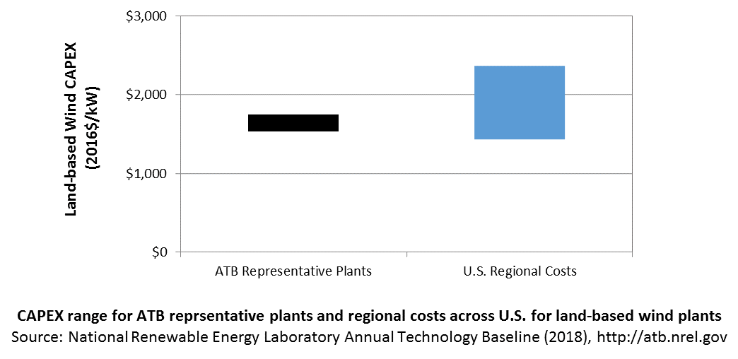
Capital expenditures (CAPEX) are expenditures required to achieve commercial operation in a given year. These expenditures include the wind turbine, the balance of system (e.g., site preparation, installation, and electrical infrastructure), and financial costs (e.g., development costs, onsite electrical equipment, and interest during construction) and are detailed in CAPEX Definition. In the ATB, CAPEX reflects typical plants and does not include differences in regional costs associated with labor, materials, taxes, or system requirements. The related Standard Scenarios product uses regional CAPEX adjustments. The range of CAPEX demonstrates variation with wind resource in the contiguous United States.
CAPEX Definition
Capital expenditures (CAPEX) are expenditures required to achieve commercial operation in a given year.
For the ATB-and based on EIA (2016a) and the System Cost Breakdown Structure defined by Moné et al. 2015 - the wind plant envelope is defined to include:
- Wind turbine supply
- Balance of system (BOS)
- Turbine installation, substructure supply, and installation
- Site preparation, installation of underground utilities, access roads, and buildings for operations and maintenance
- Electrical infrastructure, such as transformers, switchgear, and electrical system connecting turbines to each other and to the control center
- Project-related indirect costs, including engineering, distributable labor and materials, construction management start up and commissioning, and contractor overhead costs, fees, and profit.
- Financial costs
- Owners' costs, such as development costs, preliminary feasibility and engineering studies, environmental studies and permitting, legal fees, insurance costs, and property taxes during construction
- Onsite electrical equipment (e.g., switchyard), a nominal-distance spur line (< 1 mile), and necessary upgrades at a transmission substation; distance-based spur line cost (GCC) not included in the ATB
- Interest during construction estimated based on three-year duration accumulated 10%/10%/80% at half-year intervals and an 8% interest rate (ConFinFactor).
CAPEX can be determined for a plant in a specific geographic location as follows:
Regional cost variations and geographically specific grid connection costs are not included in the ATB (CapRegMult = 1; GCC = 0). In the ATB, the input value is overnight capital cost (OCC) and details to calculate interest during construction (ConFinFactor).
In the ATB, CAPEX represents a typical land-based wind plant and varies with annual average wind speed. Regional cost effects associated with labor rates, material costs, and other regional effects as defined by IEA 2016a, DOE 2015 expand the range of CAPEX. Unique land-based spur line costs for each of the 130,000 areas based on distance and transmission line costs expand the range of CAPEX even further. The figure below illustrates the ATB representative plants relative to the range of CAPEX including regional costs across the contiguous United States. Note that the ATB Base Year estimate for TRG 4 is equivalent to the market data observed capacity-weighted average wind plant CAPEX in the same year. The ATB representative plants are associated with a regional multiplier of 1.0.
Standard Scenarios Model Results
ATB CAPEX, O&M, and capacity factor assumptions for the Base Year and future projections through 2050 for Constant, Mid, and Low technology cost scenarios are used to develop the NREL Standard Scenarios using the ReEDS model. See ATB and Standard Scenarios.
CAPEX in the ATB does not represent regional variants (CapRegMult) associated with labor rates, material costs, etc., but the ReEDS model does include 134 regional multipliers (EIA 2016a).
The ReEDS model determines the land-based spur line (GCC) uniquely for each of the 130,000 areas based on distance and transmission line cost.
Natural Gas Internal Combustion Engine Vehicle
Operations and maintenance (O&M) costs depend on capacity and represent the annual fixed expenditures required to operate and maintain a wind plant, including:
- Insurance, taxes, land lease payments, and other fixed costs
- Present value and annualized large component replacement costs over technical life (e.g., blades, gearboxes, and generators)
- Scheduled and unscheduled maintenance of wind plant components, including turbines and transformers, over the technical lifetime of the plant.
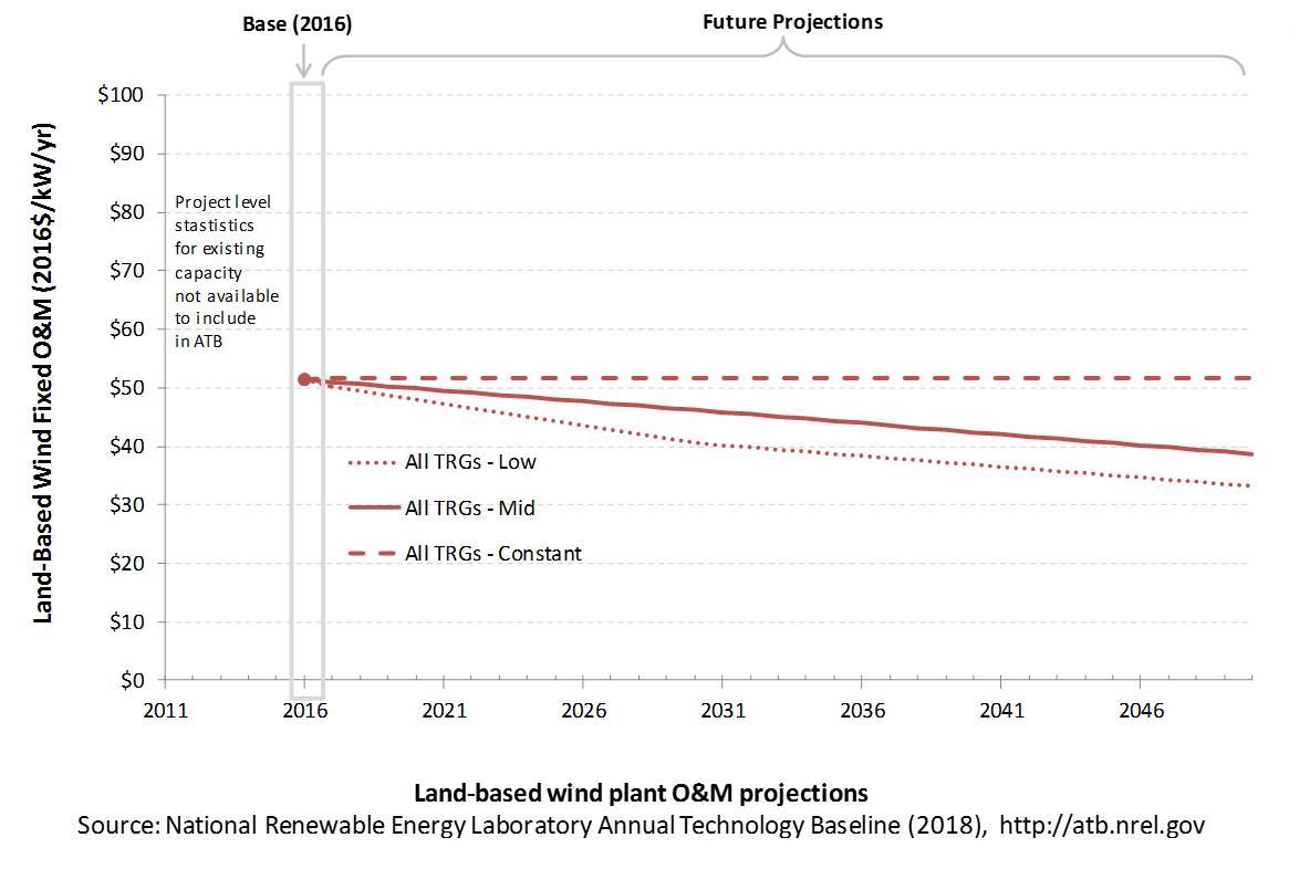
The following figure shows the Base Year estimate and future year projections for fixed O&M (FOM) costs. Three cost scenarios are represented. The estimate for a given year represents annual average FOM costs expected over the technical lifetime of a new plant that reaches commercial operation in that year.
Base Year Estimates
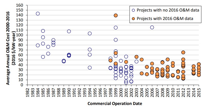
Due to limited available robust market data, an assumption of FOM of $51/kW-yr was determined to be representative of the range of available data; no variation of FOM with TRG (or wind speed) was assumed (DOE (2015)). The following chart shows sample historical data for reference.
Future Year Projections
Future FOM is assumed to decline by approximately 25% by 2050 in Mid cost case and 35% in Low cost windcases. These values are the result of linear curves fit to the results of the expert survey documented in Wiser et al. (2016).
A detailed description of the methodology for developing future year projections is found in Projections Methodology.
Technology innovations that could impact future O&M costs are summarized in LCOE Projections.
Capacity Factor: Expected Annual Average Energy Production Over Lifetime
The capacity factor represents the expected annual average energy production divided by the annual energy production, assuming the plant operates at rated capacity for every hour of the year. It is intended to represent a long-term average over the lifetime of the plant. It does not represent interannual variation in energy production. Future year estimates represent the estimated annual average capacity factor over the technical lifetime of a new plant installed in a given year.
The capacity factor is influenced by hourly windprofile, expected downtime, and energy losses within the wind plant. The specific power (ratio of machine rating to rotor swept area) and hub height are design choices that influence the capacity factor.
The following figure shows a range of capacity factors based on variation in the resource for wind plants in the contiguous United States. Historical data from wind plants operating in the United States in 2015, according to the year in which plants were installed, is shown for comparison to the ATB Base Year estimates. The range of Base Year estimates illustrate the effect of locating a wind plant in sites with high wind speeds (TRG 1) or low wind speeds (TRG 10). Future projections are shown for Constant, Mid, and Low technology cost scenarios.
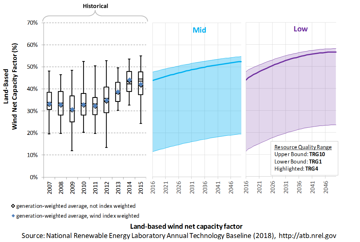
Recent Trends
Actual energy production from about 90% of wind plants operating in the United States since 2007 () is shown in box-and-whiskers format for comparison with the ATB current estimates and future projections. The historical data illustrate capacity factor for projects operating in 2016, shown by year of commercial online date. As reported in the 2016 DOE Wind Technologies Market Report (Wiser and Bolinger (2017)), NextEra Energy Resources, in their quarterly earnings reports, estimates that the "wind resource index" for the United States as a whole was 99% in 2016. The generation-weighted average 2016 capacity factors are also shown adjusted upward for a typical wind resource year by 1/0.99.
Base Year Estimates
For illustration in the ATB, all potential land-based wind plant areas were represented in 10 TRGs. The capacity-weighted average CAPEX, capacity factor, and resource potential are shown in the table below.
The majority of installed U.S. wind plants generally align with ATB estimates for performance in TRGs 5-7. High wind resource sites associated with TRGs 1 and 2 as wellas very low wind resource sites associated with TRGs 8-10 are not as common in thehistorical data, but the range of observed data encompasses ATB estimates.
The capacity factor is referenced to an 80-m, above-ground-level, long-term average hourly wind resource data fromAWS Truepower (2012).
Future Year Projections
Projections for capacity factors implicitly reflect technology innovations such as larger rotors and taller towers that will increase energy capture at the same location without specifying precise tower height or rotor diameter changes. Improvements in plant performance through lower losses and increased availability are also included implicitly.
- Mid: Projections of capacity factor for plants installed in future years were determined based on adjustments to CAPEX, FOM, and capacity factor in each year to result in a predetermined LCOEvalue.
- Low: Projections of capacity factor for plants installed in future years were determined based on the work conducted in the SMART wind power plant (Dykes et al. (2017)). The two primary factors influencing wind plant capacity factor are increased energy capture through turbine scaling and wind plant optimization. The introduction of novel control mechanisms will continue to increase energy capture with more precise control of the flow through the entire wind plant. These technology advancements are expected to increase capacity factor for all TRGs with the more aggressive increases in capacity factor happening through 2030 and then gradually becoming less aggressive through 2050.
A detailed description of the methodology for developing future year projections is found in Projections Methodology.
Technology innovations that could impact future O&M costs are summarized in LCOE Projections.
Standard Scenarios Model Results
ATB CAPEX, O&M, and capacity factor assumptions for the Base Year and future projections through 2050 for Constant, Mid, and Low technology cost scenarios are used to develop the NREL Standard Scenarios using the ReEDS model. See ATB and Standard Scenarios.
The ReEDS model output capacity factors for wind and solar PV can be lower than input capacity factors due to endogenously estimated curtailments determined by scenario constraints.
Plant Cost and Performance Projections Methodology
ATB projections were derived from two different sources for the Mid and Low cases.
- Mid: A survey of 163 of the world's wind energy experts was conducted to gain insight into possible future cost reductions, the source of those reductions, and the conditions needed to enable continued innovation and lower costs (Wiser et al. (2016)). This expert survey produced three cost reduction scenarios associated with probability levels of 10%, 50%, and 90% of achieving LCOE reductions by 2030 and 2050. In addition, the scenario results include estimated changes to CAPEX, O&M, capacity factor, project life, and weighted average cost of capital (WACC) by 2030.
- For the Mid case, the LCOE percentage reduction from the Base Year was equivalent to that corresponding to the Median Scenario (50% probability) in the expert survey (Wiser et al. (2016)).
- Expert survey estimates were normalized to the ATB Base Year starting point in order to focus on projected cost reduction instead of absolute reported costs. The percentage reductions in LCOE by 2020, 2030, and 2050 from the expert survey's Median scenario were implemented as the ATB Mid case. This is accomplished by using survey estimates for changes to capacity factor and O&M costs by 2030 and 2050. The corresponding CAPEX value to achieve the overall LCOE reduction is computed. The percentage reduction in LCOE by 2030 and by 2050 was applied equally across all TRGs. The overall reduction in LCOE by 2050 for the Mid cost scenario is approximately 31%.
- Low Technology Cost Scenario: A study conducted by NREL (Dykes et al. (2017)) assessed a variety of intelligent and novel technologies that comprise of next-generation wind plant technologies in order to estimate the LCOE of a SMART wind plant in 2030. The study used a bottom-up approach informed by research programs such as the DOE's Atmosphere to Electrons (A2e) program and input from wind energy experts to determine a future wind plant's potential LCOE impacts from enhanced power production, more efficient materials and manufacturing capabilities, lower O&M and servicing costs, lower project risks for investors, increased wind plant life, and an array of grid control and reliability features. Considering the technology advantages of the SMART wind plant, the potential for LCOE reduction is nearly doubled by 2030 compared to the Mid cost scenario derived from the expert survey, and it results in just over a 60% reduction in LCOE by 2050.
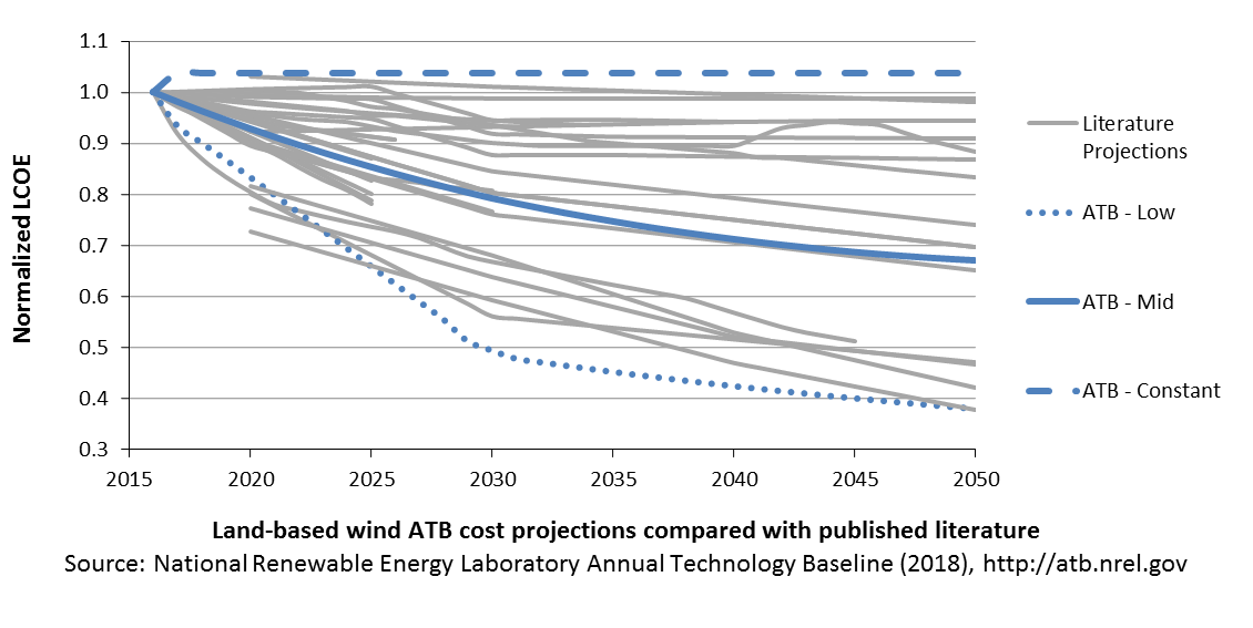
A broad sample of cost of wind energy projections is shown to provide context for the ATB Constant, Mid, and Low technology cost projections. The ATB Mid cost projection, which corresponds to the Median scenario from the expert survey, results in LCOE reductions that are slightly lower than other median scenarios in the literature (ARUP (2011); BNEF (2015); E3 (2014); EIA (2014); EPA (2015); GWEC (2014); IEA (2015c); IRENA (2016a); Teske et al. (2015)). The ATB Low cost projection, which corresponds to the NREL bottom-up cost analysis, is similar to the lower bound of the sample of literature projections (BNEF (2016); IEA (2015c); MAKE (2015)).
- Mid case projection institutions: Ove Arup & Partners Ltd., Bloomberg New Energy Finance, Energy and Environmental Economics, U.S. Energy Information Administration, United States Environmental Protection Agency, Global Wind Energy Council, International Energy Agency, International Renewable Energy Agency, and Greenpeace.
- Low case projection institutions: Bloomberg New Energy Finance, International Energy Agency, and MAKE Consulting.
Levelized Cost of Energy (LCOE) Projections
Levelized cost of energy (LCOE) is a simple metric that combines the primary technology cost and performance parameters: CAPEX, O&M, and capacity factor. It is included in the ATB for illustrative purposes. The ATB focuses on defining the primary cost and performance parameters for use in electric sector modeling or other analysis where more sophisticated comparisons among technologies are made. The LCOE accounts for the energy component of electric system planning and operation. The LCOE uses an annual average capacity factor when spreading costs over the anticipated energy generation. This annual capacity factor ignores specific operating behavior such as ramping, start-up, and shutdown that could be relevant for more detailed evaluations of generator cost and value. Electricity generation technologies have different capabilities to provide such services. For example, wind and PV are primarily energy service providers, while the other electricity generation technologies provide capacity and flexibility services in addition to energy. These capacity and flexibility services are difficult to value and depend strongly on the system in which a new generation plant is introduced. These services are represented in electric sector models such as the ReEDS model and corresponding analysis results such as the Standard Scenarios.
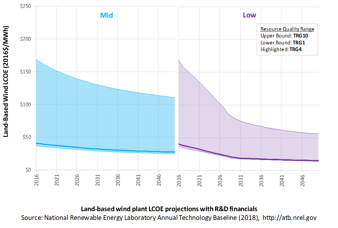
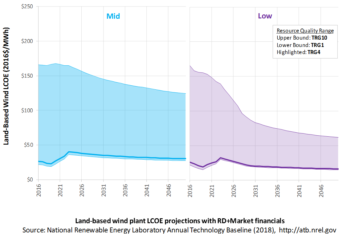
The following three figures illustrate LCOE, which includes the combined impact of CAPEX, O&M, and capacity factor projections for land-based wind across the range of resources present in the contiguous United States. For the purposes of the ATB, the costs associated with technology and project risk in the U.S. market are represented in the financing costs, not in the upfront capital costs (e.g. developer fees, contingencies). An individual technology may receive more favorable financing terms outside of the U.S., due to less technology and project risk, caused by more project development experience (e.g. offshore wind in Europe), or more government or market guarantees. The R&D Only LCOE sensitivity cases present the range of LCOE based on financial conditions that are held constant over time unless R&D affects them, and they reflect different levels of technology risk. This case excludes effects of tax reform, tax credits, technology-specific tariffs, and changing interest rates over time. The R&D + Market LCOE case adds to these the financial assumptions (1) the changes over time consistent with projections in the Annual Energy Outlook and (2) the effects of tax reform, tax credits, and tariffs. The ATB representative plant characteristics that best align with those of recently installed or anticipated near-term land-based wind plants are associated with TRG 4. Data for all the resource categories can be found in the ATB data spreadsheet.
R&D Only | R&D + Market
The methodology for representing the CAPEX, O&M, and capacity factor assumptions behind each pathway is discussed in Projections Methodology. In general, the degree of adoption of technology innovation distinguishes the Constant, Mid, and Low technology cost scenarios. These projections represent trends that reduce CAPEX and improve performance. Development of these scenarios involves technology-specific application of the following general definitions:
- Constant Technology = Base Year (or near-term estimates of projects under construction) equivalent through 2050 maintains current relative technology cost differences
- Mid Technology Cost Scenario = technology advances through continued industry growth, public and private R&D investments, and market conditions relative to current levels that may be characterized as "likely" or "not surprising"
- Low Technology Cost Scenario = Technology advances that may occur with breakthroughs, increased public and private R&D investments, and/or other market conditions that lead to cost and performance levels that may be characterized as the " limit of surprise" but not necessarily the absolute low bound.
To estimate LCOE, assumptions about the cost of capital to finance electricity generation projects are required, and the LCOE calculations are sensitive to these financial assumptions. Three project finance structures are used within the ATB:
- R&D Only Financial Assumptions: This sensitivity case allows technology-specific changes to debt interest rates, return on equity rates, and debt fraction to reflect effects of R&D on technological risk perception, but it holds background rates constant at 2016 values from AEO 2018 and excludes effects of tax reform, tax credits, and tariffs.
- R&D Only + Market Financial Assumptions: This sensitivity case retains the technology-specific changes to debt interest, return on equity rates, and debt fraction from the R&D Only case and adds in the variation over time consistent with AEO 2018, as well as effects of tax reform, tax credits, and technology-specific tariffs. For a detailed discussion of these assumptions, see Changes from 2017 ATB to 2018 ATB.
- ReEDS Financial Assumptions: ReEDS uses the R&D Only + Market Financial Assumptions for the "Mid" technology cost scenario.
A constant cost recovery period -over which the initial capital investment is recovered-is assumed for all technologies throughout this website, and can be varied in the ATB data spreadsheet.
- The equations and variables used to estimate LCOE are defined on the equations and variables page. For illustration of the impact of changing financial structures such as WACC, see Project Finance Impact on LCOE. For LCOE estimates for the Constant, Mid, and Low technology cost scenarios for all technologies, see 2018 ATB Cost and Performance Summary.
In general, differences among the technology cost cases reflect different levels of adoption of innovations. Reductions in technology costs reflect the cost reduction opportunities that are listed below.
- Continued turbine scaling to larger-megawatt turbines with larger rotors such that the swept area/megawatt capacity decreases, resulting in higher capacity factors for a given location
- Continued diversification of turbine technology whereby the largest rotor diameter turbines tend to be located in lower wind speed sites, but the number of turbine options for higher wind speed sites increases
- Taller towers that result in higher capacity factors for a given site due to the wind speed increase with elevation above ground level
- Improved plant siting and operation to reduce plant-level energy losses, resulting in higher capacity factors
- Wind turbine technology and plants that are increasingly tailored to and optimized for local site-specific conditions
- More efficient O&M procedures combined with more reliable components to reduce annual average FOM costs
- Continued manufacturing and design efficiencies such that capital cost/kilowatt decreases with larger turbine components
- Adoption of a wide range of innovative control, design, and material concepts that facilitate the above high-level trends.
Offshore Wind
Representative Technology
In 2016, the first offshore wind plant commenced commercial operation in the United States near Block Island (Rhode Island). This demonstration project is 30 MW in capacity; in the ATB, cost and performance estimates are made for commercial-scale projects 600 MW in capacity. The ATB Base Year offshore wind plant technology reflects a machine rating of 3.4 MW with a rotor diameter of 115 m and hub height of 85 m, which is typical of European projects installed in 2015-2016.
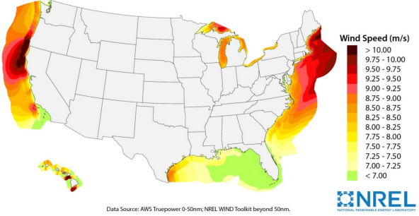
Resource Potential
Wind resource is prevalent throughout major U.S. coastal areas, including the Great Lakes. The resource potential exceeds 2,000 GW (Musial et al. (2016)), excluding Alaska. Prior estimates of offshore wind resource potential (Schwartz et al. (2010)) were updated in 2016 to extend domain boundaries from 50 nautical miles (nm) to 200 nm, consider turbine hub heights of 100 m (previously 90 m), and assume a capacity array power density of 3 MW/km2 (Musial et al. (2016)). A range of technology exclusions were applied based on maximum water depth for deployment, minimum wind speed, and limits to floating technology in freshwater surface ice. Resource potential was represented by over 7,000 areas for offshore wind plant deployment after accounting for competing use and environmental exclusions, such as marine protected areas, shipping lanes, pipelines, and others.
Source: Musial et al. 2016
Renewable energy technical potential, as defined by Lopez et al. 2012, represents the achievable energy generation of a particular technology given system performance, topographic limitations, and environmental and land-use constraints. The primary benefit of assessing technical potential is that it establishes an upper-boundary estimate of development potential. It is important to understand that there are multiple types of potential-resource, technical, economic, and market (Lopez at al. 2012; NREL, "Renewable Energy Technical Potential").
Base Year and Future Year Projections Overview
Based on the Musial et al. (2016) resource assessment, LCOE was estimated at more than 7,000 areas (with a total capacity of approximately 2,000 GW) in Beiter et al. (2016), taking into consideration a variety of spatial parameters, such as wind speeds, water depth, distance from shore, distance to ports, and wave height. CAPEX, O&M, and capacity factor are calculated for each geographic location using engineering models, hourly wind resource profiles, and representative sea states. The spatial LCOE assessment served as the basis for estimating the ATB baseline LCOE in the Base Year 2016, weighted by the available capacity, for fixed-bottom and floating offshore wind technology.
The Base Year LCOE assumes a 3.4-MW turbine size and long-term average hourly wind profiles and it reflects the least-cost choice among three substructure types (Beiter et al. (2016)):
- Monopile (fixed-bottom)
- Jacket (fixed-bottom)
- Semi-submersible (floating).
The representative offshore wind plant size is assumed to be 600 MW (Beiter et al. (2016)). For illustration in the ATB, the full resource potential, represented by 7,000 areas, was divided into 15 techno-resource groups (TRGs), of which TRGs 1-5 are representative of fixed-bottom wind technology and TRGs 6-15 are representative of floating offshore wind technology. The capacity-weighted average CAPEX, O&M, and capacity factor for each group is presented in the ATB.
Future year projections are derived from estimated cost reduction potential for offshore wind technologies based partially on elicitation of over 160 wind industry experts (Wiser et al. (2016)). Estimates for 2016-2050 were adjusted from the 2016 ATB for inflation (2015$ to $2016$). The specific scenarios are:
- Constant Technology Cost Scenario: no change in CAPEX, O&M, or capacity factor from 2015 to 2050; consistent across all renewable energy technologies in the ATB
- Mid Technology Cost Scenario: LCOE percentage reduction from the Base Year equivalent to that corresponding to the Median Scenario (50% probability) in expert survey (Wiser et al. (2016))
- Low Technology Cost Scenario: LCOE percentage reduction from the Base Year equivalent to that corresponding to the Low scenario (10% probability) in the expert survey (Wiser et al. (2016)).
CAPital EXpenditures (CAPEX): Historical Trends, Current Estimates, and Future Projections
Capital expenditures (CAPEX) are expenditures required to achieve commercial operation in a given year. These expenditures include the wind turbine, the balance of system (e.g., site preparation, installation, and electrical infrastructure), and financial costs (e.g., development costs, onsite electrical equipment, and interest during construction) and are detailed in CAPEX Definition. In the ATB, CAPEX reflects typical plants and does not include differences in regional costs associated with labor, materials, taxes, or system requirements. The related Standard Scenarios product uses regional CAPEX adjustments. The range of CAPEX demonstrates variation with wind resource in the contiguous United States.
The following figure shows the Base Year estimate and future year projections for CAPEX costs. Three cost scenarios are represented: Constant, Mid, and Low technology cost cases. Historical data from land-based wind plants installed in the United States are shown for comparison to the ATB Base Year estimates. The estimate for a given year represents CAPEX of a new plant that reaches commercial operation in that year.
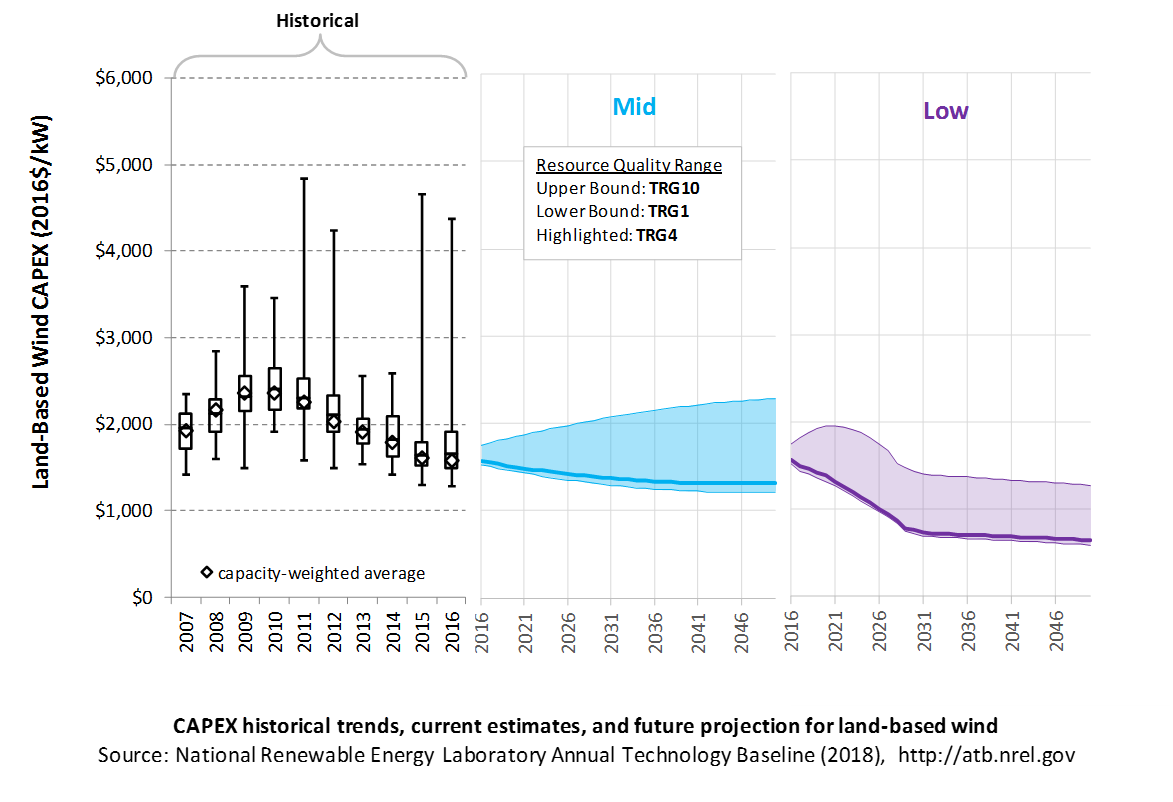
CAPEX estimates for 2016 correspond well with market data for plants installed in 2016. Projections reflect a continuation of the downward trend observed in the recent past and are anticipated to continue based on preliminary data for 2017 projects.
In the lower wind resource areas represented by TRGs 6-10, CAPEX is expected to grow as future wind turbine technology transitions to new platforms, including taller towers, larger rotors, and higher machine ratings. In the higher wind resource areas represented by TRGs 1-5, optimization of current wind turbine platforms will lead to lower CAPEX in future years.
Recent Trends
Actual land-based wind plant CAPEX (Wiser and Bolinger (2017)) is shown in box-and-whiskers format for comparison to the ATB current CAPEX estimates and future projections. provide statistical representation of CAPEX for about 65% of wind plants installed in the United States since 2007. CAPEX estimates should tend toward the low end of observed cost because no regional impacts or spur line costs are included. These effects are represented in the market data.
Base Year Estimates
For illustration in the ATB, all potential land-based wind plant areas were represented in 10 TRGs. These were defined by resource potential (GW) and have higher resolution on the highest-quality TRGs, as these are the most likely sites to be deployed, based on their economics.
TRG 1 represents the best 100 GW of wind, as determined by LCOE. TRG 2 represents the next best 200 GW, while TRG 3 represents the next best 400 GW, and TRG 4 represents the next best 800 GW. TRGs 5-9 all represent 1,600 GW of resource potential. TRG 10 represents the remaining 1,148 GW of available potential. This representation is based on the approach described in DOE (2015) and implemented with 2015 market data in Moné et al. (2017).
The following table summarizes the annual average wind speed range for each TRG, capacity-weighted average wind speed, cost and performance parameters for each TRG, and resource potential in terms of capacity and energy for each TRG. Typical land-based wind installations in 2015 and 2016 are associated with TRG4.
TRG Definitions for Land-Based Wind
| Techno-Resource Group (TRG) | Wind Speed Range (m/s) | Weighted Average Wind Speed (m/s) | Weighted Average CAPEX ($/kW) | Weighted Average OPEX ($/kW-yr) | Weighted Average Net CF (%) | Potential Wind Plant Capacity (GW) | Potential Wind Plant Energy (TWh) |
|---|---|---|---|---|---|---|---|
| TRG1 | 8.2-13.5 | 8.7 | 1,573 | 51 | 47.4% | 100 | 414 |
| TRG2 | 8.0-10.9 | 8.4 | 1,592 | 51 | 46.2% | 200 | 810 |
| TRG3 | 7.7-11.1 | 8.2 | 1,599 | 51 | 45.0% | 400 | 1,576 |
| TRG4 | 7.5-13.1 | 7.9 | 1,605 | 51 | 43.5% | 800 | 3,050 |
| TRG5 | 6.9-11.1 | 7.5 | 1,616 | 51 | 40.7% | 1,600 | 5,708 |
| TRG6 | 6.1-9.4 | 6.9 | 1,642 | 51 | 36.4% | 1,600 | 5,098 |
| TRG7 | 5.4-8.3 | 6.2 | 1,678 | 51 | 30.8% | 1,600 | 4,320 |
| TRG8 | 4.7-6.9 | 5.5 | 1,708 | 51 | 24.6% | 1,600 | 3,443 |
| TRG9 | 4.0-6.0 | 4.8 | 1,713 | 51 | 18.3% | 1,600 | 2,558 |
| TRG10 | 1.0-5.3 | 4.0 | 1,713 | 51 | 11.1% | 1,148 | 1,116 |
| Total | 10,648 | 28,092 | |||||
Future Year Projections
Mid: Projections of future LCOE were derived from a survey of wind industry experts (Wiser et al. (2016)) for scenarios that are associated with a 50% probability level in 2030 and 2050. Projections of future land-based wind plant CAPEX were determined based on adjustments to CAPEX, fixed O&M (FOM), and capacity factor in each year to result in a predetermined LCOE value derived from Wiser et al. (2016).
In order to achieve the overall LCOE reduction associated with the median and low projections from the expert survey, CAPEX was used to accommodate all improvement aspects other than O&M and capacity factor survey results. In the lower wind resource areas represented by TRGs 6-10, CAPEX is expected to grow as future wind turbine technology transitions to new platforms, including taller towers, larger rotors, and higher machine ratings. In the higher wind resource areas represented by TRGs 1-5, optimization of current wind turbine platforms will lead to lower CAPEX.
Low: Projections of future LCOE for the Low cost scenario were derived from an accelerated development pathway that included incremental improvements to technology through scaling and learning as well as innovation enabled by the DOE's Atmosphere to Electrons research program and anticipated scientific advances (Dykes et al. (2017)). The reductions in turbine and balance-of-system CAPEX were estimated by a survey of wind industry experts (Wiser et al. (2016)) focusing on detailed line item cost reduction potential. The results of the survey show a reduction in turbine and balance-of-system CAPEX by 2030 through turbine scaling with less material use and use of more efficient manufacturing processes. The accelerated decline in CAPEX is expected for all TRGs through 2030 except TRGs 9 and 10, where CAPEX is expected to slightly increase in the near term and then begin to decline at the same rate as the remaining TRGs. After 2030, the rate of CAPEX reduction is expected to continue but at a slower rate. As stated in Dykes et al. (2017), the wind turbine industry is expected to continue trends in scaling seen over the past several decades while learning processes will keep the per-unit power costs of these turbines at or below current levels. In addition, the turbine size increases will lead to economies of scale for the wind power plant through reductions in plant infrastructure and erection costs while science-enabled R&D pathways in turbine design will push materials and manufacturing costs of per-unit power to levels lower than those observed today.
A detailed description of the methodology for developing future year projections is found in Projections Methodology.
Technology innovations that could impact future O&M costs are summarized in LCOE Projections.
CAPEX Definition
Capital expenditures (CAPEX) are expenditures required to achieve commercial operation in a given year.
Based on EIA (2013), Moné et al. (2015), and Beiter et al. (2016), the System Cost Breakdown Structure of the ATB for the wind plant envelope is defined to include:
- Wind turbine supply
- Balance of system (BOS)
- Turbine installation, substructure supply and installation
- Site preparation, port and staging area support for delivery, storage, handling, and installation of underground utilities
- Electrical infrastructure, such as transformers, switchgear, and electrical system connecting turbines to each other (array cable system costs) and to the cable landfall (export cable system costs)
- Development and project management
- Financial costs
- Owners' costs, such as development costs, preliminary feasibility and engineering studies, environmental studies and permitting, legal fees, insurance costs, and property taxes during construction
- Interest during construction estimated based on three-year duration accumulated 40%/40%/20% at half-year intervals and an 8% interest rate (ConFinFactor).
CAPEX can be determined for a plant in a specific geographic location as follows:
Regional cost variations are not included in the ATB (CapRegMult = 1). In the ATB, the input value is overnight capital cost (OCC) and details to calculate interest during construction (ConFinFactor). Because transmission infrastructure between an offshore wind plant and the point at which a grid connection is made onshore is a significant component of the offshore wind plant cost, an offshore spur line cost (OffSpurCost) for each TRG is included in the CAPEX estimate. The offshore spur line cost reflects a capacity-weighted average of all potential wind plant areas within a TRG, similar to OCC.
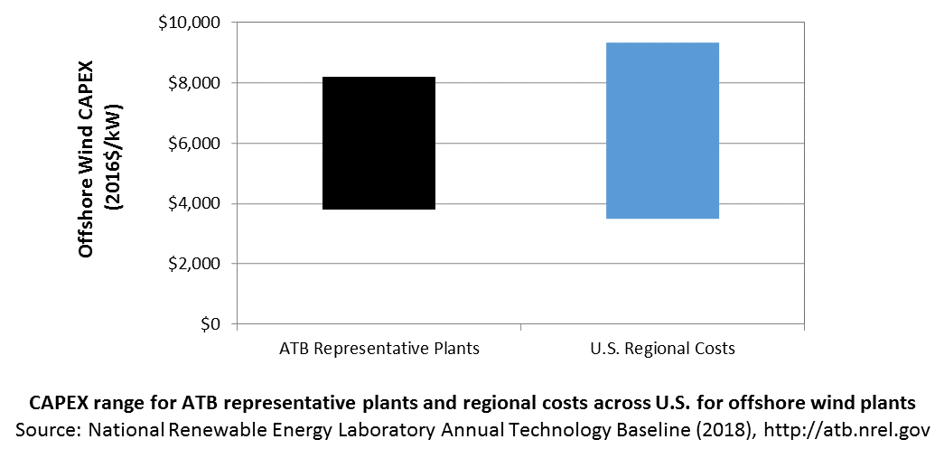
In the ATB, CAPEX represents the capacity-weighted average values of all potential wind plant areas within a TRG and varies with water depth and distance from shore. Regional cost effects associated with labor rates, material costs, and other regional effects as defined by DOE 2015 expand the range of CAPEX. Unique land-based spur line costs for each of the 7,000 areas based on distance and transmission line costs expand the range of CAPEX even further. The following figure illustrates the ATB representative plants relative to the range of CAPEX including regional costs across the contiguous United States. The ATB representative plants are associated with a regional multiplier of 1.0.
Standard Scenarios Model Results
ATB CAPEX, O&M, and capacity factor assumptions for the Base Year and future projections through 2050 for Constant, Mid, and Low technology cost scenarios are used to develop the NREL Standard Scenarios using the ReEDS model. See ATB and Standard Scenarios.
CAPEX in the ATB does not represent regional variants (CapRegMult) associated with labor rates, material costs, etc., but the ReEDS model does include 134 regional multipliers (EIA (2013)).
The ReEDS model determines offshore spur line and land-based spur line (GCC) uniquely for each of the 7,000 areas based on distance and transmission line cost.
Natural Gas Internal Combustion Engine Vehicle
Operations and maintenance (O&M) costs represent the annual fixed expenditures required to operate and maintain a wind plant over its lifetime of 30 years, including:
- Insurance, taxes, land lease payments and other fixed costs (e.g., project management and administration, weather forecasting, and condition monitoring)
- Present value and annualized large component replacement costs over technical life (e.g., blades, gearboxes, and generators)
- Scheduled and unscheduled maintenance of wind plant components, including turbines and transformers, over the technical lifetime of the plant.
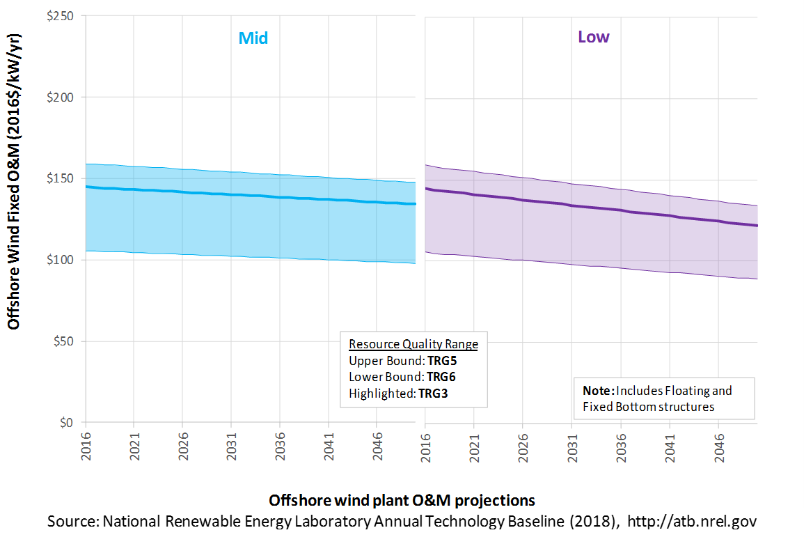
The following figure shows the Base Year estimate and future year projections for fixed O&M (FOM) costs. Three cost scenarios are represented. The estimate for a given year represents annual average FOM costs expected over the technical lifetime of a new plant that reaches commercial operation in that year. The range of Base Year O&M estimates reflects distance from shore and metocean conditions.
Base Year Estimates
FOM costs vary by distance from shore and metocean conditions. As a result, O&M costs vary from $106/kW-year (TRG 6) to $159/kW-year (TRG 5) in 2016. The capacity-weighted average in the ATB for fixed-bottom offshore technology (TRGs 1-5) is $148/kW-year; the corresponding value for floating offshore wind technology (TRGs 6-15) is $127/kW-year.
Future Year Projections
Future fixed-bottom offshore wind technology O&M is assumed to decline 7% by 2050 in the Mid cost case and 16% in the Low cost wind case, based on the expert survey conducted by Wiser et al. (2016).
Future floating offshore wind technology O&M is assumed to decline 7% by 2050 in the Mid cost case and 16% in the Low cost wind case, based on the expert survey conducted by Wiser et al. (2016).
A detailed description of the methodology for developing future year projections is found in Projections Methodology.
Technology innovations that could impact future O&M costs are summarized in LCOE Projections.
Capacity Factor: Expected Annual Average Energy Production Over Lifetime
The capacity factor represents the expected annual average energy production divided by the annual energy production, assuming the plant operates at rated capacity for every hour of the year. It is intended to represent a long-term average over the lifetime of the plant. It does not represent interannual variation in energy production. Future year estimates represent the estimated annual average capacity factor over the technical lifetime of a new plant installed in a given year.
The capacity factor is influenced by the rotor swept area/generator capacity, hub height, hourly wind profile, expected downtime, and energy losses within the wind plant. It is referenced to 100-m above-water-surface, long-term average hourly wind resource data from Musial et al. (2016).
The following figure shows a range of capacity factors based on variation in the wind resource, water depth, and distance from shore for offshore wind plants in the contiguous United States. Pre-construction estimates for offshore wind plants operating globally in 2015, according to the year in which plants were installed, is shown for comparison to the ATB Base Year estimates. The range of Base Year estimates illustrate the effect of locating an offshore wind plant in a variety of wind resource, water depth, and distance from shore conditions (TRGs 1-5 are fixed-bottom offshore wind plants and TRGs 6-15 are floating offshore wind plants). Future projections are shown for Constant, Mid, and Low technology cost scenarios.
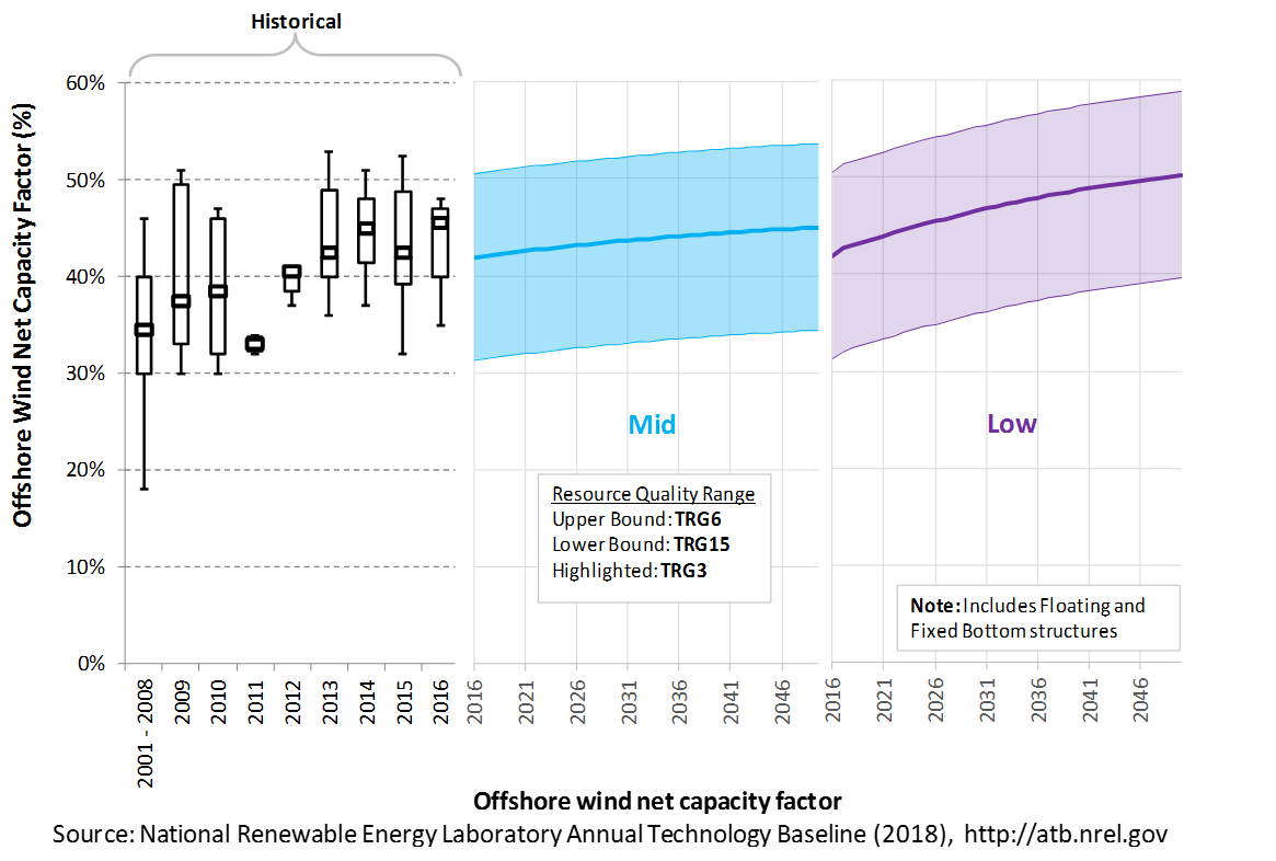
Recent Trends
Pre-construction annual energy estimates from 93% of global operating wind capacity in 2016 (NREL's internal offshore wind database) is shown in a box-and-whiskers format for comparison with the ATB current estimates and future projections. The historical data illustrate pre-construction estimated capacity factors for projects by year of commercial online date. The range of capacity factors defined by the ATB TRGs compared well with the estimated capacity factors for projects installed in 2015.
Base Year Estimates
The capacity factor is determined using a representative power curve for a generic NREL-modeled offshore wind turbine (Beiter et al. (2016)) and includes geospatial estimates of gross capacity factors for the entire resource area (Musial et al. (2016)). The net capacity factor considers spatial variation in wake losses, electrical losses, turbine availability, and other system losses. For illustration in the ATB, all 7,000 wind plant areas are represented in 15 TRGs.
TRG Definitions for Offshore Wind
| TRG | LCOE Range ($/MWh) | Wind Speed Range (m/s) | Weighted Average Wind Speed (m/s) | Weighted Water Depth (m) | Weighted Distance Site to Cable Landfall (km) | Weighted Average CAPEX ($/kW) | Weighted Average OPEX ($/kW/yr) | Weighted Average Net CF (%) | Potential Wind Plant Capacity (GW) | Potential Wind Plant Energy (TWh) |
|---|---|---|---|---|---|---|---|---|---|---|
| Fixed-Bottom | ||||||||||
| TRG 1 | LCOE <= 141 | 8.5–9.0 | 8.6 | 13 | 6 | 3,800 | 137 | 45% | 12 | 49 |
| TRG 2 | LCOE <= 149 | 8.0–8.5 | 8.4 | 16 | 9 | 3,890 | 143 | 43% | 25 | 94 |
| TRG 3 | LCOE <= 157 | 8.0–8.5 | 8.3 | 19 | 15 | 4,027 | 145 | 42% | 50 | 182 |
| TRG 4 | LCOE <= 192 | 8.0–8.5 | 8.3 | 26 | 36 | 4,556 | 152 | 40% | 320 | 1,131 |
| TRG 5 | LCOE <= 306 | 7.5–8.0 | 7.9 | 36 | 72 | 5,333 | 159 | 37% | 320 | 1,023 |
| Floating | ||||||||||
| TRG 6 | LCOE <= 166 | 9.5–10 | 9.7 | 130 | 24 | 5,961 | 105 | 51% | 12 | 55 |
| TRG 7 | LCOE <= 175 | 9.5–10 | 9.7 | 145 | 40 | 6,217 | 108 | 50% | 25 | 108 |
| TRG 8 | LCOE <= 188 | 9.5–10 | 9.5 | 139 | 50 | 6,337 | 111 | 48% | 50 | 212 |
| TRG 9 | LCOE <= 206 | 9.0–9.5 | 9.4 | 136 | 70 | 6,687 | 122 | 47% | 100 | 414 |
| TRG 10 | LCOE <= 229 | 9.0–9.5 | 9.1 | 140 | 94 | 6,931 | 129 | 45% | 200 | 781 |
| TRG 11 | LCOE <= 252 | 8.5–9.0 | 8.7 | 323 | 118 | 7,211 | 134 | 42% | 200 | 727 |
| TRG 12 | LCOE <= 274 | 8.0–8.5 | 8.1 | 404 | 123 | 7,224 | 135 | 37% | 200 | 651 |
| TRG 13 | LCOE <= 299 | 7.5–8.0 | 7.8 | 474 | 138 | 7,411 | 136 | 35% | 200 | 615 |
| TRG 14 | LCOE <= 341 | 7.0–7.5 | 7.4 | 615 | 130 | 7,606 | 131 | 32% | 200 | 566 |
| TRG 15 | LCOE <= 438 | 7.5–8.0 | 7.5 | 797 | 199 | 8,204 | 138 | 31% | 143 | 390 |
| Total | 2,058 | 6,997 | ||||||||
Future Year Projections
Projections of capacity factors for plants installed in future years were determined based on estimates obtained through an expert survey conducted by Wiser et al. (2016) for both fixed-bottom and floating offshore wind technologies. Projections for capacity factors implicitly reflect technology innovations such as larger rotors and taller towers that will increase energy capture at the same geographic location without explicitly specifying tower height and rotor diameter changes.
A detailed description of the methodology for developing future year projections is found in Projections Methodology.
Technology innovations that could impact future O&M costs are summarized in LCOE Projections.
Standard Scenarios Model Results
ATB CAPEX, O&M, and capacity factor assumptions for the Base Year and future projections through 2050 for Constant, Mid, and Low technology cost scenarios are used to develop the NREL Standard Scenarios using the ReEDS model. See ATB and Standard Scenarios.
The ReEDS model output capacity factors for offshore wind can be lower than input capacity factors due to endogenously estimated curtailments determined by scenario constraints.
Plant Cost and Performance Projections Methodology
ATB projections were derived from the results of a survey of 163 of the world's wind energy experts Wiser et al. (2016). The survey was conducted to gain insight into the possible future cost reductions, the source of those reductions, and the conditions needed to enable continued innovation and lower costs (Wiser et al. (2016)). The expert survey produced three cost reduction scenarios associated with probability levels of 10%, 50%, and 90% of achieving LCOE reductions by 2030 and 2050. In addition, the scenario results include estimated changes to CAPEX, O&M, capacity factor, project life, and weighted average cost of capital (WACC) by 2030.
For the ATB, three different technology cost scenarios were adapted from the expert survey results for scenario modeling as bounding levels:
- Constant Technology Cost Scenario: no change in CAPEX, O&M, or capacity factor from 2015 to 2050; consistent across all renewable energy technologies in the ATB
- Mid Technology Cost Scenario: LCOE percentage reduction from the Base Year equivalent to that corresponding to the Median Scenario (50% probability) in the expert survey (Wiser et al. (2016))
- Low Technology Cost Scenario: LCOE percentage reduction from the Base Year equivalent to that corresponding to the Low scenario (10% probability) in the expert survey (Wiser et al. (2016)).
Expert survey estimates were normalized to the ATB Base Year starting point in order to focus on projected cost reduction instead of absolute reported costs. The percentage reduction in LCOE by 2020, 2030, and 2050 from the expert survey's Median and Low scenarios are implemented as the ATB Mid and Low cost scenarios. This is accomplished by utilizing survey estimates for changes to capacity factor and O&M costs by 2030 and 2050. The corresponding CAPEX value to achieve the overall LCOE reduction is computed. The percentage reduction in LCOE by 2030 and by 2050 was applied equally across all TRGs. The overall reduction in LCOE by 2050 for the Mid cost scenario is 39% and for the Low cost scenario is 51%.
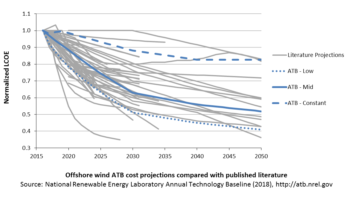
A broad sample of cost of offshore wind energy projections provides context for the ATB Constant, Mid, and Low technology cost projections. Based on a TRG4 resource classification,[1] the ATB Mid cost projection, which corresponds to the median scenario from the Wiser et al. (2016) expert survey, results in LCOE reductions that are fairly aligned with the median scenarios of external studies (BNEF (2017c); IRENA (2016b); Catapult (2016); Lazard (2017)). EIA (2017b) estimates higher cost levels in the period 2022-2041, while BNEF (2018) estimates lower cost levels for the U.S by the mid-2020s. These external studies were reviewed to validate the baseline estimates and projections derived for the ATB. Generally, while some published studies as well as recent tender awards for European projects to be installed by the mid-2020s suggest significant near-term cost reduction (see e.g., Musial et al. (2017)), it is likely that the United States will lag due to a different development stage of the U.S. supply chain and port infrastructure.
The relative costs of mid-depth water plants and deep water, or floating, offshore wind plants are maintained constant throughout the scenarios for simplicity. Some hypothesize that unique aspects of floating technologies, such as the ability to assemble and commission turbines at the port, could reduce the cost of floating technologies relative to fixed-bottom technologies.
Levelized Cost of Energy (LCOE) Projections
Levelized cost of energy (LCOE) is a simple metric that combines the primary technology cost and performance parameters: CAPEX, O&M, and capacity factor. It is included in the ATB for illustrative purposes. The ATB focuses on defining the primary cost and performance parameters for use in electric sector modeling or other analysis where more sophisticated comparisons among technologies are made. The LCOE accounts for the energy component of electric system planning and operation. The LCOE uses an annual average capacity factor when spreading costs over the anticipated energy generation. This annual capacity factor ignores specific operating behavior such as ramping, start-up, and shutdown that could be relevant for more detailed evaluations of generator cost and value. Electricity generation technologies have different capabilities to provide such services. For example, wind and PV are primarily energy service providers, while the other electricity generation technologies provide capacity and flexibility services in addition to energy. These capacity and flexibility services are difficult to value and depend strongly on the system in which a new generation plant is introduced. These services are represented in electric sector models such as the ReEDS model and corresponding analysis results such as the Standard Scenarios.
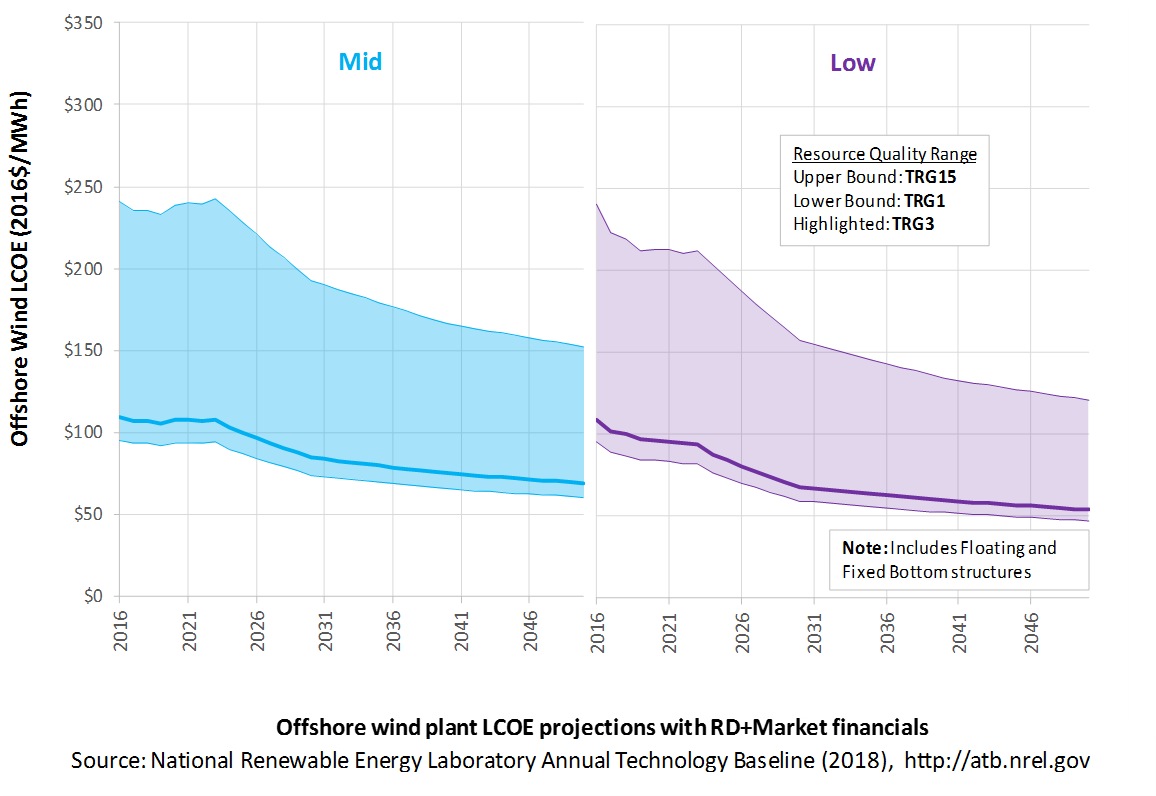
The following three figures illustrate LCOE, which includes the combined impact of CAPEX, O&M, and capacity factor projections for off-shore wind across the range of resources present in the contiguous United States. For the purposes of the ATB, the costs associated with technology and project risk in the U.S. market are represented in the financing costs, not in the upfront capital costs (e.g. developer fees, contingencies). An individual technology may receive more favorable financing terms outside of the U.S., due to less technology and project risk, caused by more project development experience (e.g. offshore wind in Europe), or more government or market guarantees. The R&D Only LCOE sensitivity cases present the range of LCOE based on financial conditions that are held constant over time unless R&D affects them, and they reflect different levels of technology risk. This case excludes effects of tax reform, tax credits, technology-specific tariffs, and changing interest rates over time. The R&D + Market LCOE case adds to these the financial assumptions (1) the changes over time consistent with projections in the Annual Energy Outlook and (2) the effects of tax reform, tax credits, and tariffs. The ATB representative plant characteristics that best align with those of recently installed or anticipated near-term land-based wind plants are associated with TRG 4. Data for all the resource categories can be found in the ATB data spreadsheet.
R&D Only | R&D + Market
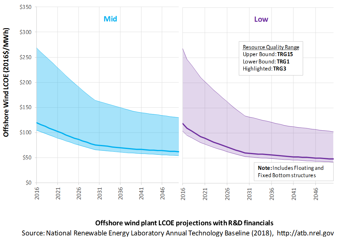
The methodology for representing the CAPEX, O&M, and capacity factor assumptions behind each pathway is discussed in Projections Methodology. In general, the degree of adoption of technology innovation distinguishes the Constant, Mid, and Low technology cost scenarios. These projections represent trends that reduce CAPEX and improve performance. Development of these scenarios involves technology-specific application of the following general definitions:
- Constant Technology = Base Year (or near-term estimates of projects under construction) equivalent through 2050 maintains current relative technology cost differences
- Mid Technology Cost Scenario = technology advances through continued industry growth, public and private R&D investments, and market conditions relative to current levels that may be characterized as "likely" or "not surprising"
- Low Technology Cost Scenario = Technology advances that may occur with breakthroughs, increased public and private R&D investments, and/or other market conditions that lead to cost and performance levels that may be characterized as the " limit of surprise" but not necessarily the absolute low bound.
- To estimate LCOE, assumptions about the cost of capital to finance electricity generation projects are required, and the LCOE calculations are sensitive to these financial assumptions. Three project finance structures are used within the ATB:
- R&D Only Financial Assumptions: This sensitivity case allows technology-specific changes to debt interest rates, return on equity rates, and debt fraction to reflect effects of R&D on technological risk perception, but it holds background rates constant at 2016 values from AEO 2018 and excludes effects of tax reform, tax credits, and tariffs.
- R&D Only + Market Financial Assumptions: This sensitivity case retains the technology-specific changes to debt interest, return on equity rates, and debt fraction from the R&D Only case and adds in the variation over time consistent with AEO 2018, as well as effects of tax reform, tax credits, and technology-specific tariffs. For a detailed discussion of these assumptions, see Changes from 2017 ATB to 2018 ATB.
- ReEDS Financial Assumptions: ReEDS uses the R&D Only + Market Financial Assumptions for the "Mid" technology cost scenario.
- A constant cost recovery period -over which the initial capital investment is recovered-is assumed for all technologies throughout this website, and can be varied in the ATB data spreadsheet.
- The equations and variables used to estimate LCOE are defined on the equations and variables page. For illustration of the impact of changing financial structures such as WACC, see Project Finance Impact on LCOE. For LCOE estimates for the Constant, Mid, and Low technology cost scenarios for all technologies, see 2018 ATB Cost and Performance Summary.
- In general, differences among the technology cost cases reflect different levels of adoption of innovations. Reductions in technology costs reflect the cost reduction opportunities that are listed below.
- Continued turbine scaling to larger-megawatt turbines with larger rotors such that swept area/megawatt capacity decreases resulting in higher capacity factors for a given location
- Greater market competition in the production of primary components (e.g., turbines, support structure), and installation services
- Economy-of-scale and productivity improvements in manufacturing, including mass production of substructure component and optimized installation strategies
- Improved plant siting and operation to reduce plant-level energy losses, resulting in higher capacity factors
- More efficient O&M procedures combined with more reliable components to reduce annual average FOM costs
- Adoption of a wide range of innovative control, design, and material concepts that facilitate the high-level trends described above.
Geothermal
Geothermal technology cost and performance projections will be more extensively updated upon completion of the Geothermal Vision Study. Until then, the projections are based on those documented in 2017 ATB - Geothermal, with the following changes:
- The dollar year was updated from 2015 to 2016 with 1.3% inflation.
- Technology-specific financial assumptions are included, as for other technologies in 2018 ATB, using data from Wall 2017.
Reference: Wall, A. M., Pl Dobson, H. Thomas (2017). "Geothermal Costs of Capital: Relating Market Valuation to Project Risk and Technology." Geothermal Resources Council Transactions, v. 41. https://www.geothermal-library.org/index.php?mode=pubs&action=view&record=1033704.
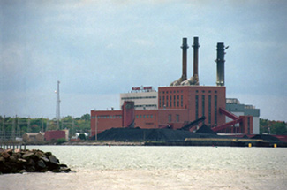
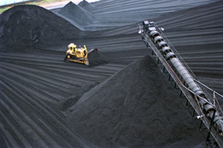
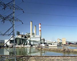
Coal
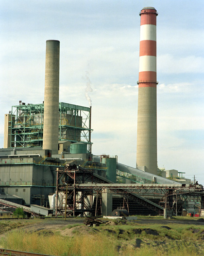
In a coal power plant:
- Heat is created: Coal is pulverized, mixed with hot air, and burned in suspension.
- Water turns to steam: The heat turns purified water into steam, which is piped to the turbine.
- Steam turns the turbine: The pressure of the steam pushes the turbine blade, turns the shaft in the generator, and creates power.
- Steam is turned back into water: Cool water is drawn into a condenser where the steam turns back into water that can be used over again in the plant.
The process outlined above is adapted from Duke Energy ("How Energy Works"). Coal plant emissions and performance are also impacted by the kind of coal (coal rank) that the plant burns. Lignite, subbituminous, bituminous, and anthracite coal all are of varying quality. The amount of moisture, sulfur, and ash in a particular type of coal can have significant influence on coal plant operation, design, and cost.
(soon to be set up for cofiring biomass)
Renewable energy technical potential, as defined by Lopez et al. 2012, represents the achievable energy generation of a particular technology given system performance, topographic limitations, and environmental and land-use constraints. Technical resource potential corresponds most closely to fossil reserves, as both can be characterized by the prospect of commercial feasibility and depend strongly on available technology at the time of the resource assessment. Coal reserves in the United States are assessed by the United States Geological Survey (USGS, "Coal Assessments").
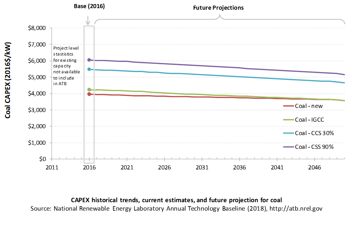
CAPital EXpenditures (CAPEX): Historical Trends, Current Estimates, and Future Projections
Technology cost and performance projections are taken from the AEO Reference Scenario (EIA 2017). Because little-to-no coal is built in the Reference Scenario, coal capital expenditures (CAPEX) decline according to the minimum learning rate. Pulverized coal is a relatively mature technology, and therefore has a low minimum learning rate. Integrated gasification combined cycle (IGCC) technology, where the coal is gasified and then fed into a combined cycle turbine, is less mature and is assumed to have a slightly higher minimum learning rate. Coal with carbon capture and storage (CCS) is also a newer technology with a higher minimum learning rate.
Comparison with Other Sources
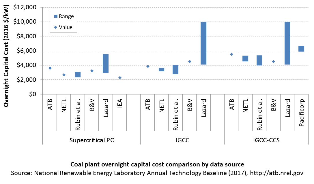
Lazard (2016) does not explicitly define their ranges with and without CCS; thus, the high end of their pulverized coal and IGCC ranges and the low end of their IGCC-CCS range are assumed to be the middle of the full reported range. All sources have been normalized to the same dollar year. Costs vary due to differences in system design (e.g., coal rank), methodology, and plant cost definitions. The coal capital costs include environmental controls to meet current federal regulations.
CAPEX Definition
Capital expenditures (CAPEX) are expenditures required to achieve commercial operation in a given year.
For coal power plants, CAPEX equals interest during construction (ConFinFactor) times the overnight capital cost (OCC).
Overnight capital costs are modified from EIA (2017). Capital costs include overnight capital cost plus defined transmission cost, and it removes a material price index.
Fuel costs, which are just passed through to end user, are taken from EIA (2017).
For the ATB, coal-CCS technology is ultra-supercritical pulverized coal technology fitted with CCS. Both 30% capture and 90% capture options are included for the coal-CCS technology. The CCS plant configuration includes only the cost of capturing and compressing the CO2. It does not include CO2 delivery and storage.
| Overnight Capital Cost ($/kW) | Construction Financing Factor (ConFinFactor) | CAPEX ($/kW) | |
|---|---|---|---|
| Coal-new:Ultra-supercritical pulverized coal with SO2 and NOx controls | $3.559 | 1.084 | $3,859 |
| Coal-IGCC:Integrated gasification combined cycle (IGCC) | $3,819 | 1.084 | $4,141 |
| Coal-CCS:Ultra-supercritical pulverized coal with carbon capture and sequestration (CCS) options (30% / 90% capture) | $4,927 / $5,448 | 1.084 | $5,341 / $5,906 |
CAPEX can be determined for a plant in a specific geographic location as follows:
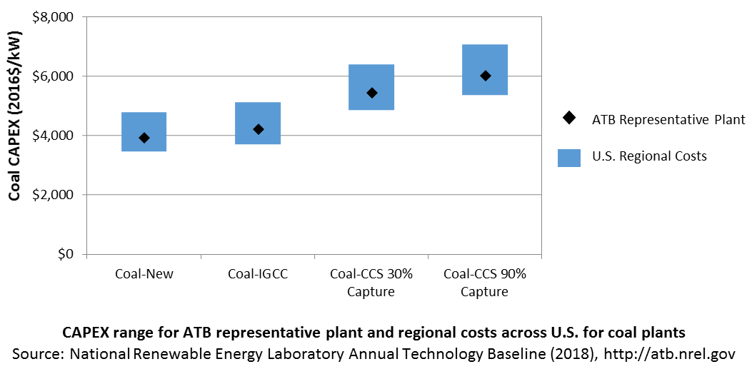
Regional cost variations and geographically specific grid connection costs are not included in the ATB (CapRegMult = 1; GCC = 0). In the ATB, the input value is overnight capital cost (OCC) and details to calculate interest during construction (ConFinFactor).
In the ATB, CAPEX represents each type of a coal plant with a unique value. Regional cost effects associated with labor rates, material costs, and other regional effects as defined by EIA 2016a expand the range of CAPEX. Unique land-based spur line costs based on distance and transmission line costs are not estimated. The following figure illustrates the ATB representative plant relative to the range of CAPEX including regional costs across the contiguous United States. The ATB representative plants are associated with a regional multiplier of 1.0.
Natural Gas Internal Combustion Engine Vehicle
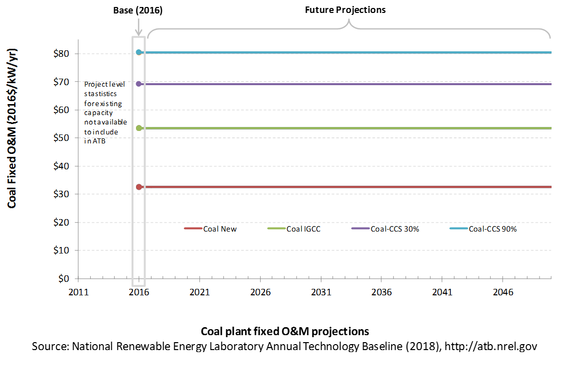
Operations and maintenance (O&M) costs represent the annual expenditures required to operate and maintain a plant over its lifetime, including:
- Insurance, taxes, land lease payments, and other fixed costs
- Present value and annualized large component replacement costs over technical life
- Scheduled and unscheduled maintenance of power plants, transformers, and other components over the technical lifetime of the plant.
Market data for comparison are limited and generally inconsistent in the range of costs covered and the length of the historical record.
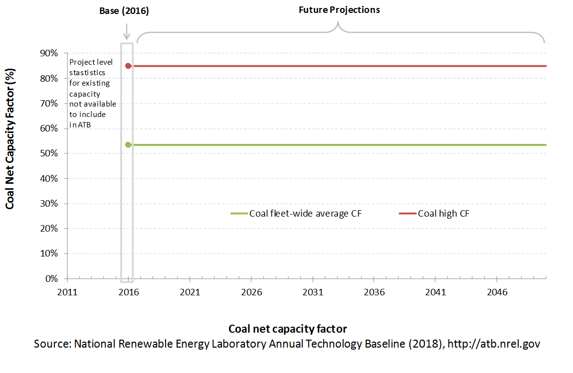
Capacity Factor: Expected Annual Average Energy Production Over Lifetime
The capacity factor represents the assumed annual energy production divided by the totalpossible annual energy production, assuming the plant operates at rated capacity for every hour of the year. For coal plants, the capacity factors are typically lower than their availability factors. Coal plant availability factors have a wide range depending on system design and maintenance schedules.
The capacity factor of dispatchable units is typically a function of the unit's marginal costs and local grid needs (e.g., need for voltage support or limits due to transmission congestion).
Coal power plants have typically been operated as baseload units, although that has changed in many locations due to low natural gas prices and increased penetration of variable renewable technologies. The average capacity factor used in the ATB is the fleet-wide average reported by EIA for 2015. The high capacity factor represents a new plant that would operate as a baseload unit.
Even though IGCC and coal with CCS have experienced limited deployment in the United States, it is expected that their performance characteristics would be similar to new coal power plants.
Levelized Cost of Energy (LCOE) Projections
Levelized cost of energy (LCOE) is a simple metric that combines the primary technology cost and performance parameters: CAPEX, O&M, and capacity factor. It is included in the ATB for illustrative purposes. The ATB focuses on defining the primary cost and performance parameters for use in electric sector modeling or other analysis where more sophisticated comparisons among technologies are made. The LCOE accounts for the energy component of electric system planning and operation. The LCOE uses an annual average capacity factor when spreading costs over the anticipated energy generation. This annual capacity factor ignores specific operating behavior such as ramping, start-up, and shutdown that could be relevant for more detailed evaluations of generator cost and value. Electricity generation technologies have different capabilities to provide such services. For example, wind and PV are primarily energy service providers, while the other electricity generation technologies provide capacity and flexibility services in addition to energy. These capacity and flexibility services are difficult to value and depend strongly on the system in which a new generation plant is introduced. These services are represented in electric sector models such as the ReEDS model and corresponding analysis results such as the Standard Scenarios.
References
2H 2017 Offshore Wind Market Outlook. Presentation by Tom Harries, accessed through BNEF subscription services.
Annual Energy Outlook 2017 with Projections to 2050. Washington, D.C.: U.S. Department of Energy. January 5, 2017. http://www.eia.gov/outlooks/aeo/pdf/0383(2017).pdf.
Energy Technology Perspectives 2015.
Innovation Outlook: Off shore Wind. Abu Dhabi: International Renewable Energy Agency.
Lazard's Levelized Cost of Energy Analysis: Version 11.0. November 2017. New York: Lazard. https://www.lazard.com/perspective/levelized-cost-of-energy-2017.
Levelized Cost and Levelized Avoided Cost of New Generation Resources in the Annual Energy Outlook 2017.
The Power to Change: Solar and Wind Cost Reduction Potential to 2025. June 2016. Paris: International Renewable Energy Agency. http://www.irena.org/DocumentDownloads/Publications/IRENA_Power_to_Change_2016.pdf.
U.S. Offshore Wind. Presentation by Tom Harries, accessed through BNEF subscription services.
AWS Truepower. 2012. Wind Resource of the United States: Mean Annual Wind Speed at 200m Resolution. https://www.awstruepower.com/assets/Wind-Resource-Map-UNITED-STATES-11x171.pdf.
B&V (Black & Veatch). 2012. Cost and Performance Data for Power Generation Technologies. Black & Veatch Corporation. February 2012. http://bv.com/docs/reports-studies/nrel-cost-report.pdf.
Beiter, Philipp, Walter Musial, Aaron Smith, Levi Kilcher, Rick Damiani, Michael Maness, Senu Sirnivas, Tyler Stehly, Vahan Gevorgian, Meghan Mooney, and George Scott. 2016. A Spatial-Economic Cost-Reduction Pathway Analysis for U.S. Offshore Wind Energy Development from 2015-2030. Golden, CO: National Renewable Energy Laboratory. NREL/TP-6A20-66579. September 2016. http://www.nrel.gov/docs/fy16osti/66579.pdf.
BNEF (Bloomberg New Energy Finance). 2015. Future Cost of Wind.
Catapult. 2016. Cost Reduction Monitoring Framework. Quantitative Assessment Report. 19 December 2016.
DOE (U.S. Department of Energy). 2015. Wind Vision: A New Era for Wind Power in the United States. U.S. Department of Energy. DOE/GO-102015-4557. March 2015. http://energy.gov/sites/prod/files/2015/03/f20/wv_full_report.pdf.
Dykes, K., M. Hand, T. Stehly, P. Veers, M. Robinson, E. Lantz. 2017. Enabling the SMART Wind Power Plant of the Future Through Science-Based Innovation (Technical Report), NREL/TP-5000-68123. National Renewable Energy Laboratory (NREL). Golden, CO (US). https://www.nrel.gov/docs/fy17osti/68123.pdf.
E3 (Energy and Environmental Economics). 2014. Capital Cost Review of Power Generation Technologies: Recommendations for WECC's 10- and 20-Year Studies. Prepared for the Western Electric Coordinating Council. https://www.wecc.biz/Reliability/2014_TEPPC_Generation_CapCost_Report_E3.pdf.
EIA (U.S. Energy Information Administration). 2013. Updated Capital Cost Estimates for Utility Scale Electricity Generating Plants. Washington, D.C.: U.S. Department of Energy, U.S. Energy Information Administration. https://www.eia.gov/outlooks/capitalcost/pdf/updated_capcost.pdf.
EIA (U.S. Energy Information Administration). 2014. Annual Energy Outlook 2014 with Projections to 2040. Washington, D.C.: U.S. Department of Energy. DOE/EIA-0383(2014). April 2014. http://www.eia.gov/forecasts/aeo/pdf/0383(2014).pdf.
EIA (U.S. Energy Information Administration). 2016a. Capital Cost Estimates for Utility Scale Electricity Generating Plants. Washington, D.C.: U.S. Department of Energy. November 2016. https://www.eia.gov/analysis/studies/powerplants/capitalcost/pdf/capcost_assumption.pdf.
EIA (U.S. Energy Information Administration). 2018. Annual Energy Outlook 2018 with Projections to 2050. Washington, D.C.: U.S. Department of Energy. February 6, 2018. https://www.eia.gov/outlooks/aeo/pdf/AEO2018.pdf.
EPA (United States Environmental Protection Agency). Clean Power Plan.
Global Wind Energy Council (GWEC). 2014. Global Wind Energy Outlook 2014. October 2014.
IEA (International Energy Agency). 2016. World Energy Outlook 2016. Paris: International Energy Agency. December 2016.
Lazard. 2016. Levelized Cost of Energy Analysis-Version 10.0. December 2016. New York: Lazard. https://www.lazard.com/media/438038/levelized-cost-of-energy-v100.pdf.
Lopez, Anthony, Billy Roberts, Donna Heimiller, Nate Blair, and Gian Porro. 2012. U.S. Renewable Energy Technical Potentials: A GIS-Based Analysis. National Renewable Energy Laboratory. NREL/TP-6A20-51946. http://www.nrel.gov/docs/fy12osti/51946.pdf.
MAKE Consulting (MAKE). 2015. Global Wind Power Supply Chain. Market Report. December 2015.
Moné, C., A. Smith, M. Hand, and B. Maples. 2015. 2013 Cost of Wind Energy Review. Golden, CO: National Renewable Energy Laboratory. http://www.nrel.gov/docs/fy15osti/63267.pdf.
Moné, Christopher, Maureen Hand, Mark Bolinger, Joseph Rand, Donna Heimiller, and Jonathan Ho. 2017. 2015 Cost of Wind Energy Review. Golden, CO: National Renewable Energy Laboratory. NREL/TP-6A20-66861. http://www.nrel.gov/docs/fy17osti/66861.pdf.
Musial, W., P. Beiter, P. Schwabe, T. Tian, T. Stehly, P. Spitsen. 2017. 2016 Offshore Wind Technologies Market Report. U.S. Department of Energy Office of Energy Efficiency and Renewable Energy. DOE/GO-102017-5031. August 2017. https://www.energy.gov/sites/prod/files/2018/08/f35/2016%20Offshore%20Wind%20Technologies%20Market%20Report.pdf
Musial, Walt, Donna Heimiller, Philipp Beiter, George Scott, and Caroline Draxl. 2016. 2016 Offshore Wind Energy Resource Assessment for the United States. Golden, CO: National Renewable Energy Laboratory. NREL/TP-5000-66599. September 2016. http://www.nrel.gov/docs/fy16osti/66599.pdf.
NETL (National Energy Technology Laboratory: Tim Fout, Alexander Zoelle, Dale Keairns, Marc Turner, Mark Woods, Norma Kuehn, Vasant Shah, Vincent Chou, Lora Pinkerton). 2015. Fossil Energy Plants: Volume 1a: Bituminous Coal (PC) and Natural Gas to Electricity, Revision 3. DOE/NETL-2015/1723. http://www.netl.doe.gov/File%20Library/Research/Energy%20Analysis/Publications/Rev3Vol1aPC_NGCC_final.pdf.
NREL (National Renewable Energy Laboratory). 2012. Renewable Electricity Futures Study. Hand, M.M., S. Baldwin, E. DeMeo, J.M. Reilly, T. Mai, D. Arent, G. Porro, M. Meshek, and D. Sandor, eds. 4 vols. NREL/TP-6A20-52409. Golden, CO: National Renewable Energy Laboratory. https://www.nrel.gov/analysis/re-futures.html.
Ove Arup & Partners Ltd. (ARUP). 2011. Review of the Generation Costs and Deployment Potential of Renewable Electricity Technologies in the UK. Department of Energy and Climate REP001, Prepared by Ove Arup & Partners Ltd. London, UK.
Rubin, Edward S., John E. Davison, and Howard J. Herzog. 2015. "The Cost of CO2 Capture and Storage." International Journal of Greenhouse Gas Control 40(September 2015): 378–400. http://www.sciencedirect.com/science/article/pii/S1750583615001814, preprint available at http://www.cmu.edu/epp/iecm/rubin/PDF%20files/2015/Rubin_et_al_ThecostofCCS_IJGGC_2015.pdf.
Schwartz, Marc, Donna Heimiller, Steve Haymes, and Walt Musial. 2010. Assessment of Offshore Wind Energy Resources for the United States. Golden, CO: National Renewable Energy Laboratory. NREL/TP-500-45889. June 2010. http://www.nrel.gov/docs/fy10osti/45889.pdf.
Teske, Sven, Steve Sawyer, and Oliver Schäfer, Thomas Pregger, Sonja Simon, and Tobias Naegler. 2015. Energy [r]evolution: A Sustainable World Energy Outlook 2015. Global Wind Energy Council, Solar Power Europe & Greenpeace. September 2015.
Wiser, Ryan, and Mark Bolinger. 2014. 2014 Wind Technologies Market Report. U.S. Department of Energy. DOE/GO-102015-4702. https://energy.gov/sites/prod/files/2015/08/f25/2014-Wind-Technologies-Market-Report-8.7.pdf.
Wiser, Ryan, and Mark Bolinger. 2017. 2016 Wind Technologies Market Report. https://www.energy.gov/sites/prod/files/2017/10/f37/2016_Wind_Technologies_Market_Report_101317.pdf.
Wiser, Ryan, Karen Jenni, Joachim Seel, Erin Baker, Maureen Hand, Eric Lantz, and Aaron Smith. 2016. Forecasting Wind Energy Costs and Cost Drivers: The Views of the World's Leading Experts. Berkeley, CA: Lawrence Berkeley National Laboratory. LBNL-1005717. June 2016. https://emp.lbl.gov/publications/forecasting-wind-energy-costs-and.