Annual Technology Baseline 2018
National Renewable Energy Laboratory
Recommended Citation:
NREL (National Renewable Energy Laboratory). 2018. 2018 Annual Technology Baseline. Golden, CO: National Renewable Energy Laboratory. http://atb.nrel.gov/.
Please consult Guidelines for Using ATB Data:
https://atb.nrel.gov/electricity/user-guidance.html
Utility-Scale PV
Representative Technology
Utility-scale PV systems in the ATB are representative of one-axis tracking systems with performance and pricing characteristics in line with a 1.3 DC-to-AC ratio-or inverter loading ratio (ILR) (Fu et al. (2017)). PV system performance characteristics in previous ATB versions were designed in the ReEDS model at a time when PV system ILRs were lower than they are in current system designs; performance and pricing in the 2018 ATB incorporates more up-to-date system designs and therefore assumes a higher ILR.
Resource Potential
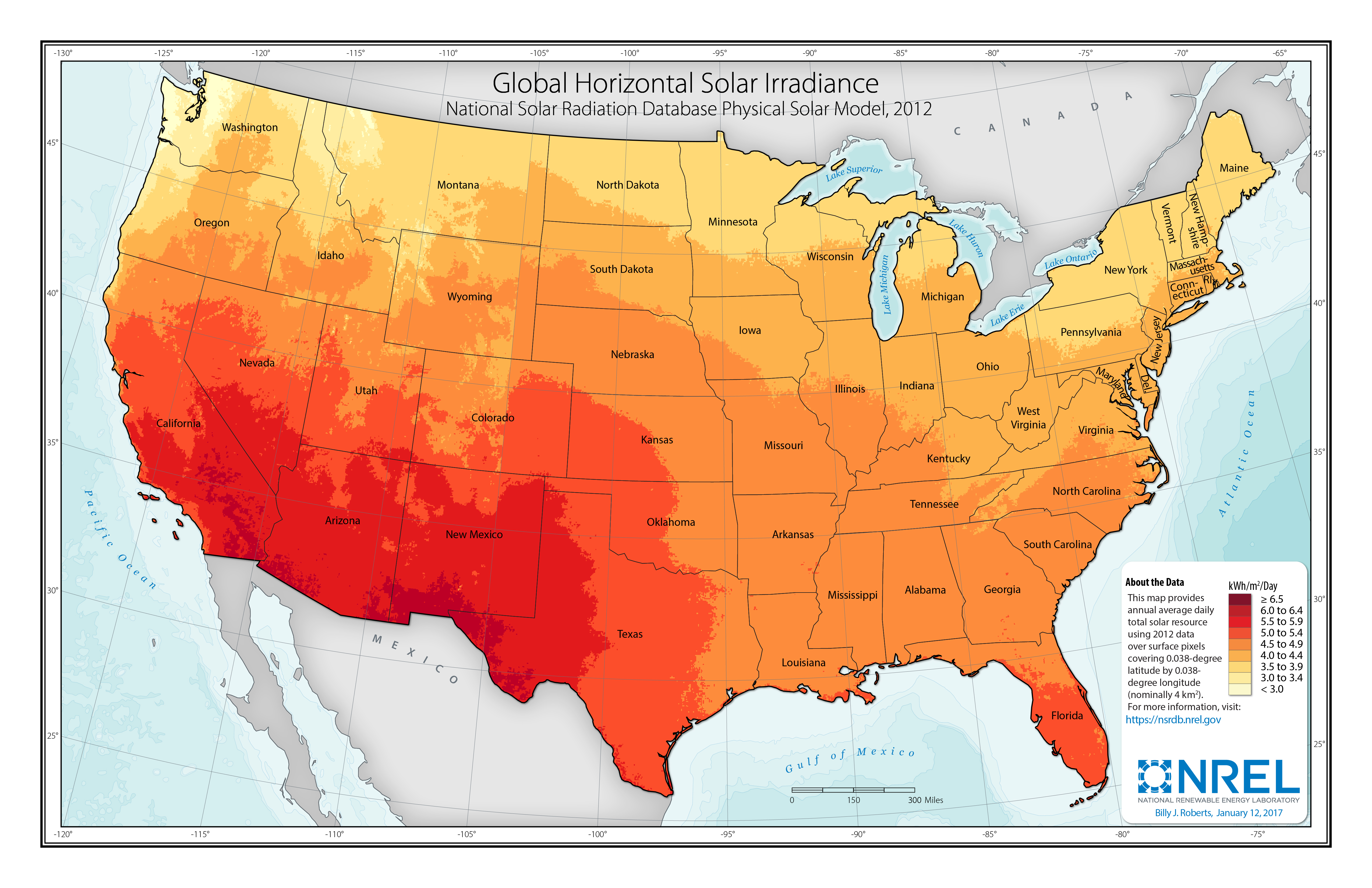
Solar resources across the United States are mostly good to excellent at about 1,000-2,500 kWh/m2/year. The Southwest is at the top of this range, while Alaska and part of Washington are at the low end. The range for the contiguous United States is about 1,350-2,500 kWh/m2/year. Nationwide, solar resource levels vary by about a factor of two.
The total U.S. land area suitable for PV is significant and will not limit PV deployment. One estimate (Denholm and Margolis (2008)) suggests the land area required to supply all end-use electricity in the United States using PV is about 5,500,000 hectares (ha) (13,600,000 acres), which is equivalent to 0.6% of the country's land area or about 22% of the " urban area" footprint (this calculation is based on deployment/land in all 50states).
Renewable energy technical potential, as defined by Lopez et al. 2012, represents the achievable energy generation of a particular technology given system performance, topographic limitations, and environmental and land-use constraints. The primary benefit of assessing technical potential is that it establishes an upper-boundary estimate of development potential. It is important to understand that there are multiple types of potential-resource, technical, economic, and market (Lopez at al. 2012; NREL, "Renewable Energy Technical Potential").
Base Year and Future Year Projections Overview
The Base Year estimates rely on modeled CAPEX and O&M estimates benchmarked with industry and historical data. Capacity factor is estimated based on hours of sunlight at latitude for all geographiclocations in the United States. The ATB presents capacity factor estimates that encompass a range associated with Low, Mid,and Constant technology cost scenarios across the United States.
Future year projections are derived from analysis of published projections of PV CAPEX and bottom-up engineering analysis of O&M costs. Three different projections were developed for scenario modeling as bounding levels:
- Constant Technology Cost Scenario: no change in CAPEX, O&M, or capacity factor from 2017 to 2050; consistent across all renewable energy technologies in the ATB
- Mid Technology Cost Scenario: based on the median of literature projections of future CAPEX; O&M technology pathway analysis
- Low Technology Cost Scenario: based on the low bound of literature projections of future CAPEX and O&M technology pathway analysis.
CAPital EXpenditures (CAPEX): Historical Trends, Current Estimates, and Future Projections
Capital expenditures (CAPEX) are expenditures required to achieve commercial operation in a given year. These expenditures include the hardware, the balance of system (e.g., site preparation, installation, and electrical infrastructure), and financial costs (e.g., development costs, onsite electrical equipment, and interest during construction) and are detailed in CAPEX Definition. In the ATB, CAPEX reflects typical plants and does not include differences in regional costs associated with labor, materials, taxes, or system requirements. The related Standard Scenarios product uses regional CAPEX adjustments. The range of CAPEX demonstrates variation with resource in the contiguous United States.
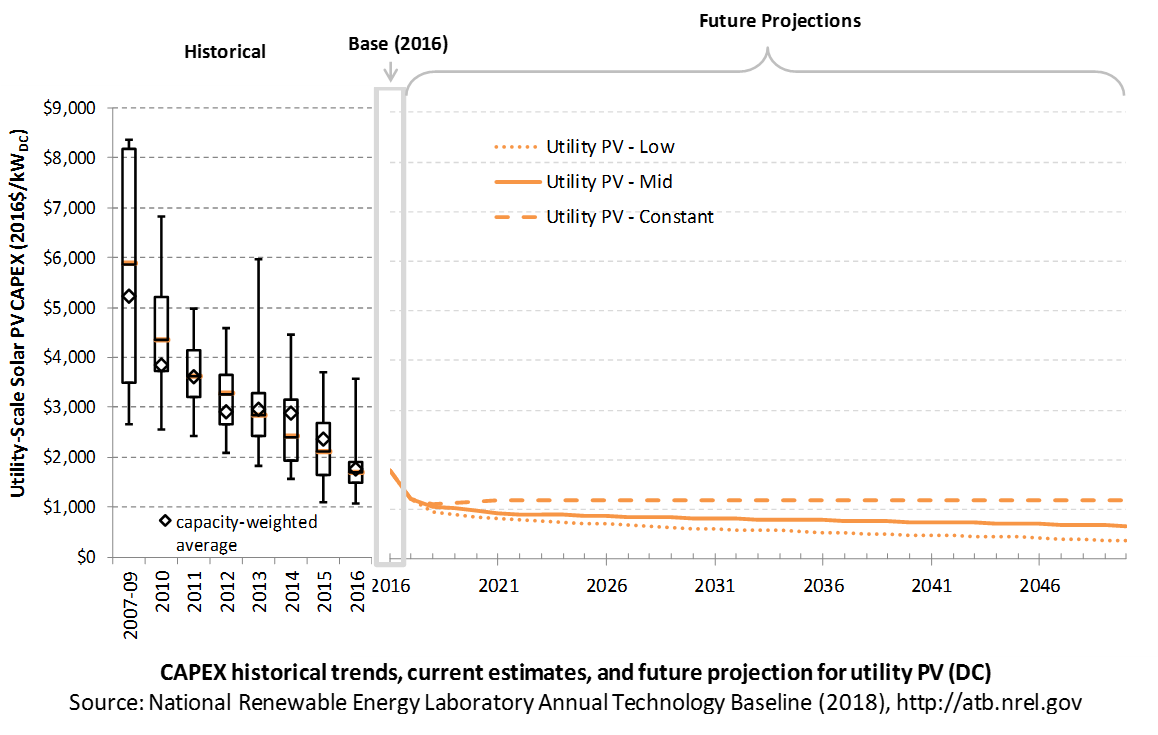
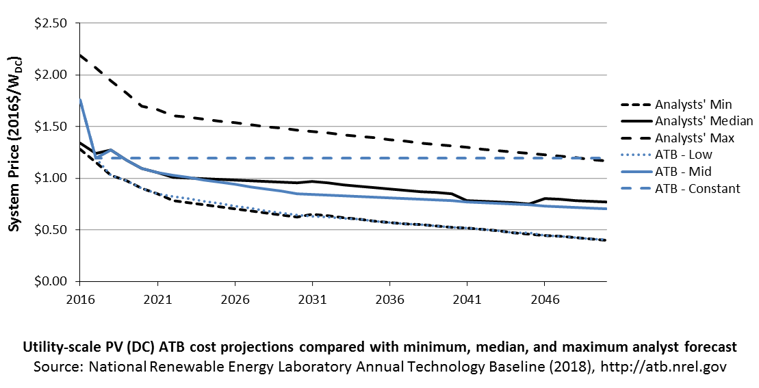
The following figures show the Base Year estimate and future year projections for CAPEX costs in terms of $/kWDC or $/kWAC. Three cost scenarios are represented: Constant, Mid, and Low technology cost. Historical data from utility-scale PV plants installed in the United States are shown for comparison to the ATB Base Year estimates. The estimate for a given year represents CAPEX of a new plant that reaches commercial operation in that year.
The PV industry typically refers to PV CAPEX in terms of $/kWDC based on the aggregated module capacity. The electric utility industry typically refers to PV CAPEX in terms of $/kWAC based on the aggregated inverter capacity. See Solar PV AC-DC Translation for details. The figures illustrate the CAPEX historical trends, current estimates, and future projections in terms of $/kWDC or $/kWAC; current estimates and future projections assume an inverter loading ratio of 1.3 while historical numbers represent reported values.
Recent Trends
Reported historical utility-scale PV plant CAPEX (Bolinger et al. (2017)) is shown in box-and-whiskers format for comparison to the ATB current CAPEX estimates and future projections. Bolinger et al. (2017) provide statistical representation of CAPEX for 88% of all utility-scale PV capacity.
PV pricing and capacities are quoted in kWDC (i.e., module rated capacity) unlike other generation technologies, which are quoted in kWAC. For PV, this would correspond to the combined rated capacity of all inverters. This is done because kWDC is the unit that most of the PV industry uses. Although costs are reported in kWDC, the total CAPEX includes the cost of the inverter, which has a capacity measured in kWAC.
CAPEX estimates for 2016 reflect continued rapid decline supported by analysis of recent power purchase agreement pricing (Bolinger et al. (2017)) for projects that will become operational in 2016 and beyond.
Base Year Estimates
For illustration in the ATB, a representative utility-scale PV plant is shown. Although the PV technologies vary, typical plant costs are represented with a single estimate because the CAPEX does not vary with solar resource.
Although the technology market share may shift over time with new developments, the typical plant cost is represented with the projections above.
A system price of $1.75/WDC in 2016 represents the capacity-weighted average price of a utility-scale PV system installed in 2016 as reported in Bolinger et al. (2017) and adjusted to remove regional cost multipliers based on geographic location of projects installed in 2016. The $1.20/WDC price in 2017 is based on modeled pricing for one-axis tracking systems quoted in Q1 2017 as reported in Fu et al. (2017), adjusted for inflation, and accounting for $0.1/W higher than expected module prices due to tariff concerns in the R&D + Market sensitivity case. These figures are in line with other estimated system prices reported in Feldman et al. (2017).
The Base Year CAPEX estimates should tend toward the low end of reported pricing because no regional impacts, time-lagged system prices, or spur line costs are included. These effects are represented in the historical market data.
For example, in 2014, the reported capacity-weighted average system price was higher than 80% of system prices in 2014 due to very large systems, with multi-year construction schedules, installed in that year. Developers of these large systems negotiated contracts and installed portions of their systems when module and other costs were higher.
Future Year Projections
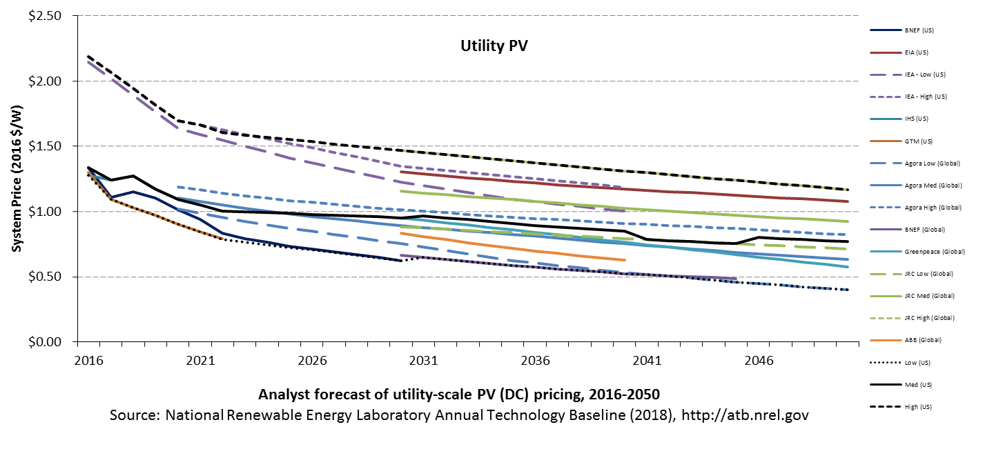
Projections of future utility-scale PV plant CAPEX are based on 15 system price projections from 9 separate institutions with short-term projections (BNEF (2017a); GTM Research (2016); EIA (2017a); EIA (2016a); IHS (2017)) (BNEF (2017a); GTM Research (2016); EIA 2017; IEA (2016); IHS (2017) made in the past year and long-term projections (ABB (2017); BNEF (2017b); Carlsson et al. (2014); Fraunhofer ISE (2015); Teske et al. (2015)) made in the last four years. We adjusted the " min," " median," and " max" projections in a few different ways. All 2016 pricing is based on the capacity-weighted average utility-scale system price as reported in Utility-Scale Solar 2016 (Bolinger et al. (2017)) and adjusted by the ReEDS state-level capital cost multipliers to remove geographic price distortions from 2016 reported pricing. All 2017 pricing is based on the bottom-up benchmark analysis reported in U.S. Solar Photovoltaic System Cost Benchmark Q1 2017 (adjusted for inflation, and accounting for $0.1/W higher than expected module prices due to tariff concerns in the R&D + Market sensitivity case) (Fu et al. (2017)). These figures are in line with other estimated system prices reported in Feldman et al. (2017).
We adjusted the Mid and Low projections for 2018-2050 to remove distortions caused by the combination of forecasts with different time horizons and based on internal judgment of price trends. In addition, because the projections were made before the Section 201 proclamation implementing a tariff on imported PV modules and cells, we adjusted projections to incorporate Section 201 tariff per pricing from internal NREL analysis in the R&D + Market sensitivity case. The Constant cost scenario is kept constant at the 2017 CAPEX value, assuming no improvements beyond2017.
The largest annual reductions in CAPEX for the Mid and Low projections occur from 2016 to 2017, dropping 32%. While reported CAPEX values have not been collected for all systems built in 2017 and 2018, historical CAPEX information has been consistent with utility-scale benchmarks after adjusting for installation data and system size.
Initial reported pricing for utility-scale power purchase agreements (PPAs) placed in service in 2016 fell to approximately $60/MWh, which is consistent in price with PPAs executed in 2013 and 2014, representing a two- to three-year lag from execution to installation. The capacity average executed PPA price in 2016 was approximately $35/MWh. If PPAs executed in 2016 follow a similar two-year lag, we would expect those systems to be installed in 2018-2019; therefore, we could see the capacity-weighted average PPA price for systems installed in the year fall from $60/MWh in 2016 to $35/MWh in 2018, or 41% less. The capacity average executed PPA price in 2016 was 41% lower than the capacity-weighted average PPA price for a system installed in 2016. While PPA pricing and CAPEX are not perfectly correlated, from 2010 to 2016, the capacity-weighted average PPA price and CAPEX for systems installed in that year fell 63% and 54% respectively (Bolinger et al. (2017)).
A detailed description of the methodology for developing future year projections is found in Projections Methodology.
Technology innovations that could impact future CAPEX costs are summarized in LCOE Projections.
CAPEX Definition
Capital expenditures (CAPEX) are expenditures required to achieve commercial operation in a given year.
For the ATB-and based on EIA (2016a) and the NREL Solar PV Cost Model (Fu et al. (2017))-the utility-scale solar PV plant envelope is defined to include:
- Hardware
- Module supply
- Power electronics, including inverters
- Racking
- Foundation
- AC and DC wiring materials and installation
- Electrical infrastructure, such as transformers, switchgear, and electrical system connecting modules to each other and to the control center
- Balance of system (BOS)
- Land acquisition, site preparation, installation of underground utilities, access roads, fencing, and buildings for operations and maintenance
- Project indirect costs, including costs related to engineering, distributable labor and materials, construction management start up and commissioning, and contractor overhead costs, fees, and profit
- Financial Costs
- Owners' costs, such as development costs, preliminary feasibility and engineering studies, environmental studies and permitting, legal fees, insurance costs, and property taxes during construction
- Electrical interconnection, including onsite electrical equipment (e.g., switchyard), a nominal-distance spur line (< 1 mile), and necessary upgrades at a transmission substation; distance-based spur line cost (GCC) not included in the ATB
- Interest during construction estimated based on six-month duration accumulated 100% at half-year intervals and an 8% interest rate (ConFinFactor).
CAPEX can be determined for a plant in a specific geographic location as follows:
Regional cost variations and geographically specific grid connection costs are not included in the ATB (CapRegMult = 1; GCC = 0). In the ATB, the input value is overnight capital cost (OCC) and details to calculate interest during construction (ConFinFactor).
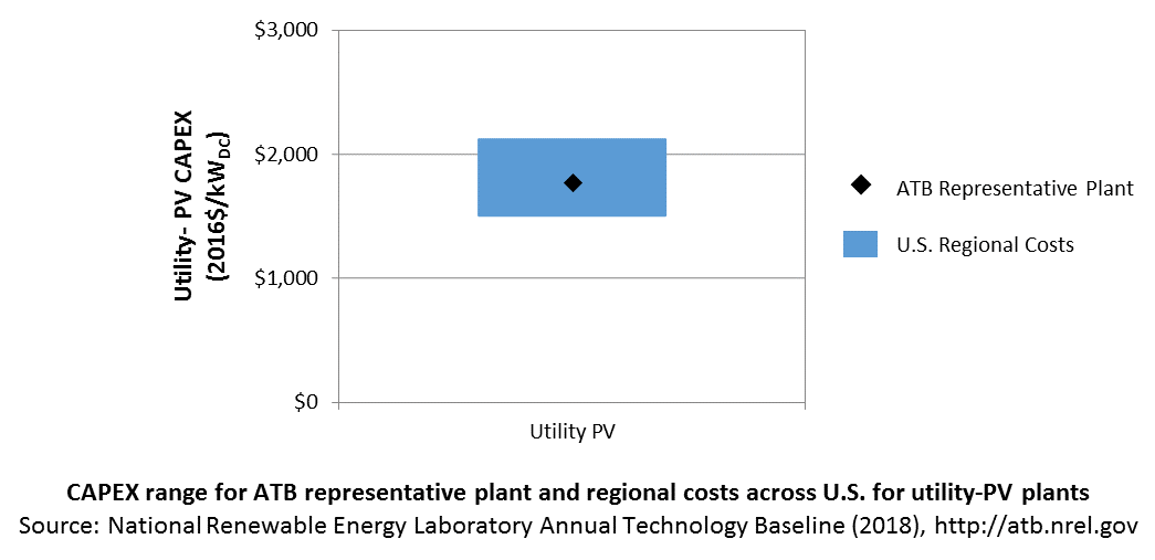
In the ATB, CAPEX represents a typical one-axis utility-scale PV plant and does not vary with resource. The difference in cost between tracking and non-tracking systems has been reduced greatly in the United States. Regional cost effects associated with labor rates, material costs, and other regional effects as defined by EIA 2016a expand the range of CAPEX. Unique land-based spur line costs based on distance and transmission line costs for potential utility-PV plant locations expand the range of CAPEX even further. The following figure illustrates the ATB representative plant relative to the range of CAPEX including regional costs across the contiguous United States. The ATB representative plants are associated with a regional multiplier of 1.0.
Standard Scenarios Model Results
ATB CAPEX, O&M, and capacity factor assumptions for the Base Year and future projections through 2050 for Constant, Mid, and Low technology cost scenarios are used to develop the NREL Standard Scenarios using the ReEDS model. See ATB and Standard Scenarios.
CAPEX in the ATB does not represent regional variants (CapRegMult) associated with labor rates, material costs, etc., but the ReEDS model does include 134 regional multipliers (EIA 2016a).
CAPEX in the ATB does not include a geographically determined spur line (GCC) from plant to transmission grid, but the ReEDS model calculates a unique value for each potential PV plant.
Natural Gas Internal Combustion Engine Vehicle
Operations and maintenance (O&M) costs represent the annual fixed expenditures required to operate and maintain a solar PV plant over its lifetime of 30 years, including:
- Insurance, property taxes, site security, legal and administrative fees, and other fixed costs
- Present value and annualized large component replacement costs over technical life (e.g., inverters at 15 years)
- Scheduled and unscheduled maintenance of solar PV plants, transformers, etc. over the technical lifetime of the plant (e.g., general maintenance, including cleaning and vegetation removal).
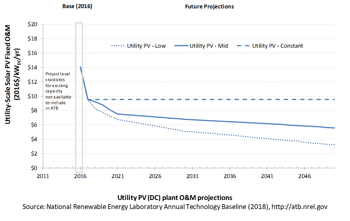
The following figure shows the Base Year estimate and future year projections for fixed O&M (FOM) costs. Three cost scenarios are represented. The estimate for a given year represents annual average FOM costs expected over the technical lifetime of a new plant that reaches commercial operation in that year.
Base Year Estimates
FOM of $14/kWDC - yr is based on the average ratio of O&M costs to CAPEX costs, 0.8%, as reported in Lazard (2017). This ratio is slightly higher than the ratio of O&M costs to historically reported CAPEX costs of 0.6%, which are derived from 2011 to 2016 historical data reported in Bolinger et al. (2017) but are lower than the ratio of O&M costs to CAPEX costs of 1.0%, which are derived from IEA (2016). A wide range in reported prices exists in the market, in part depending on the maintenance practices that exist for a particular system. These cost categories include asset management (including compliance and reporting for incentive payments), different insurance products, site security, cleaning, vegetation removal, and failure of components. Not all these practices are performed for each system; additionally, some factors depend on the quality of the parts and construction. NREL analysts estimate O&M costs can from $0 to $40/kWDC - yr.
Future Year Projections
We derive future FOM based on the same 0.8% ratio of O&M to CAPEX, used to estimate Base Year O&M costs. Historically reported data suggest O&M and CAPEX cost reductions are correlated; from 2011 to 2016, fleetwide average O&M and CAPEX costs fell 43% and 33% respectively, as reported in Bolinger et al. (2017).
A detailed description of the methodology for developing future year projections is found in Projections Methodology.
Technology innovations that could impact future O&M costs are summarized in LCOE Projections.
Capacity Factor: Expected Annual Average Energy Production Over Lifetime
The capacity factor represents the expected annual average energy production divided by the annual energy production, assuming the plant operates at rated capacity for every hour of the year. It is intended to represent a long-term average over the lifetime of the plant. It does not represent interannual variation in energy production. Future year estimates represent the estimated annual average capacity factor over the technical lifetime of a new plant installed in a given year.
Other technologies' capacity factors are represented in exclusively AC units; however, because PV pricing in this ATB documentation is represented in $/kWDC, PV system capacity is a DC rating. The PV capacity factor is the ratio of annual average energy production (kWhAC) to annual energy production assuming the plant operates at rated DC capacity for every hour of the year. For more information, see Solar PV AC-DC Translation.
The capacity factor is influenced by the hourly solar profile, technology (e.g., thin-film versus crystalline silicon), axistype (e.g., none, one, or two), expected downtime, and inverter losses to transform from DC to ACpower. The DC-AC ratio is a design choice that influences the capacity factor. PV plant capacity factor incorporates an assumed degradation rate of 0.75%/year (Fu et al. (2017)) in the annual average calculation. R&D could lower degradation rates of PV plant capacity factor; future projections for Mid and Low cost scenarios reduce degradation rates by 2050, using a straight-line basis, to 0.5%/year and 0.3%/year respectively.
The following figure shows a range of capacity factors based on variation in solar resource in the contiguous United States. The range of the Base Year estimates illustrate the effect of locating a utility-scale PV plant in places with lower or higher solar irradiance. These five values use specific locations as examples of high (Daggett, California), high-mid (Los Angeles, California), mid (Kansas City, Missouri), low-mid (Chicago, Illinois), and low (Seattle, Washington) resource areas in the United States as implemented in the SAM model using PV system characteristics from Fu et al. (2017).
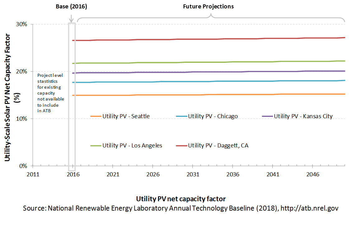
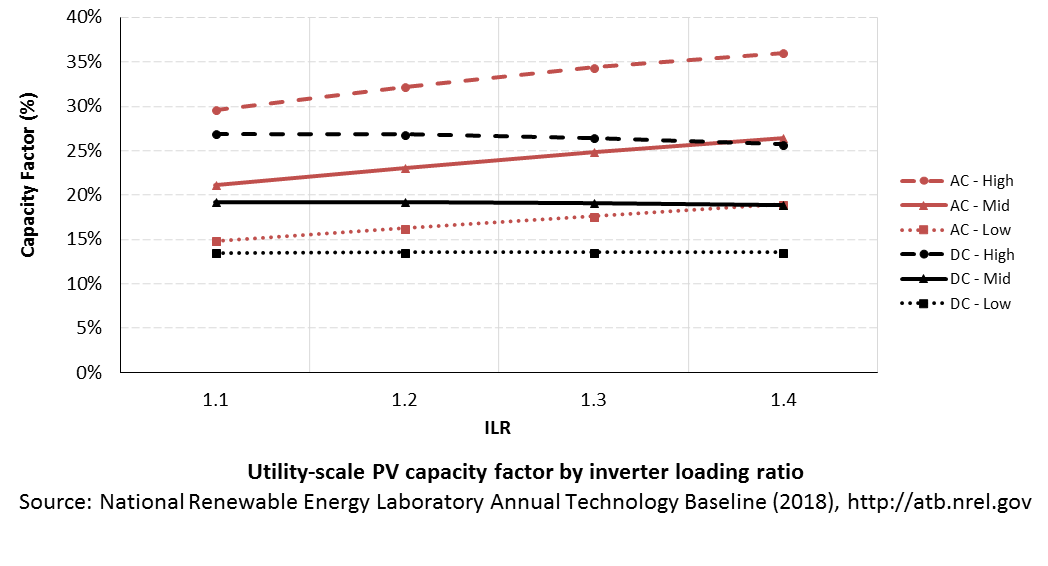
PV system inverters, which convert DC energy/power to AC energy/power, have AC capacity ratings; therefore, the capacity of a PV system is rated in MWAC, or the aggregation of all inverters' rated capacities, or MWDC, or the aggregation of all modules' rated capacities. The capacity factor calculation uses a system's rated capacity, and therefore, capacity factor can be represented using exclusively AC units or using AC units for electricity (the numerator) and DC units for capacity (the denominator). Both capacity factors will result in the same LCOE as long as the other variables use the same capacity rating (e.g., CAPEX in terms of $/kWDC). PV systems' DC ratings are typically higher than their AC ratings; therefore, the capacity factor calculated using a DC capacity rating has a higher denominator. In the ATB, we use capacity factors of 15.9%, 18.9%, 21.0%, 23.2%, and 28.3% for the first year of a PV project and adjust the values to reflect an average capacity factor for the lifetime of a project, calculated with MWDC, assuming 0.75% module capacity degradation per year in the base year and declining to 0.5% and 0.3% module capacity degradation per year by 2050 for the Mid and Low cost scenarios. The adjusted average capacity factor values used in the ATB Base Year are 14.9%, 17.7%, 19.7%, 21.7%, and 26.6%. These numbers would change to approximately 19.4%, 23.0%, 25.6%, 29.3%, and 34.5% if the ATB used MWAC. The following figure illustrates capacity factor-both DC and AC-for a range of inverter loading ratios. The ATB capacity factor assumptions are based on ILR = 1.3.
Recent Trends
At the end of 2016, the capacity-weighted average AC capacity factor for all U.S. projects installed at the time was 27.3% (including fixed-tilt systems), but individual project-level capacity factors exhibited a wide range (15.4%-35.5%).
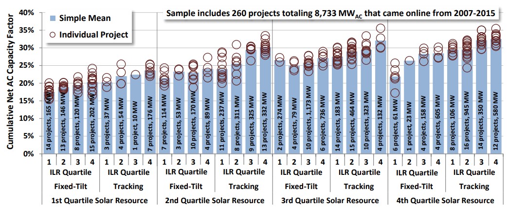
The capacity-weighted average capacity factor was more closely in line with the higher end of the range because 62% of installed capacity from the data set was placed in service in the past two years of when the data were collected (and therefore have not degraded substantially), and 82% of the installed capacity was in the southwestern United States or California, where the average capacity factor was 29.9% for one-axis systems and 25.5% for fixed-tilt systems (Bolinger et al. (2017)).
Base Year Estimates
For illustration in the ATB, a range of capacity factors associated with the range of latitude in the contiguous United States is shown.
Over time, PV plant output is reduced. This degradation (at 0.75%) is accounted for in ATB estimates of capacity factor. The ATB capacity factor estimates represent estimated annual average energy production over the 30-year lifetime.
These DC capacity factors are for a one-axis tracking system with a DC-to-AC ratio of1.3.
Future Year Projections
Projections of capacity factors for plants installed in future years are unchanged from the Base Year for the Constant cost scenario. Capacity factors for Mid and Low cost scenarios are projected to increase over time, caused by a straight-line reduction in PV plant capacity degradation rates from 0.75%, reaching 0.5%/year and 0.3%/year by 2050 for the Mid and Low cost scenarios respectively. The following table summarizes the difference in average capacity factor in 2050 caused by different degradation rates in the Constant, Mid, and Low cost scenarios.
| Seattle, WA | Chicago, IL | Kansas City, MO | Los Angeles, CA | Daggett, CA | |
|---|---|---|---|---|---|
| Low Cost (0.30% degradation rate) | 15.5% | 18.4% | 20.5% | 22.6% | 27.6% |
| Mid Cost (0.50% degradation rate) | 15.2% | 18.1% | 20.1% | 22.2% | 27.1% |
| Constant Cost (0.75% degradation rate) | 14.9% | 17.7% | 19.7% | 21.7% | 26.6% |
Solar PV plants have very little downtime, inverter efficiency is already optimized, and tracking is already assumed. That said, there is potential for future increases in capacity factors through technological improvements beyond lower degradation rates, such as less panel reflectivity and improved performance in low-light conditions.
Standard Scenarios Model Results
ATB CAPEX, O&M, and capacity factor assumptions for the Base Year and future projections through 2050 for Constant, Mid, and Low technology cost scenarios are used to develop the NREL Standard Scenarios using the ReEDS model. See ATB and Standard Scenarios.
The ReEDS model output capacity factors for wind and solar PV can be lower than input capacity factors due to endogenously estimated curtailments determined by system operation.
Plant Cost and Performance Projections Methodology
Currently, CAPEX-not LCOE-is the most common metric for PV cost. Due to differing assumptions in long-term incentives, system location and production characteristics, and cost of capital, LCOE can be confusing and often incomparable between differing estimates. While CAPEX also has many assumptions and interpretations, it involves fewer variables to manage. Therefore, PV projections in the ATB are driven primarily by CAPEX cost improvements, along with minor improvements in operational cost and cost of capital.
The Constant, Mid, and Low technology cost cases explore the range of possible outcomes of future PV cost improvements:
- Constant: no improvements made beyond today
- Mid: current expectations of price reductions in a " business-as-usual" scenario
- Low: expectations of potential cost reductions given improved R&D funding, favorable financing, and more aggressive global deployment targets.
While CAPEX is one of the drivers to lower costs, R&D efforts continue to focus on other areas to lower the cost of energy from utility-scale PV, such as longer system lifetime and improved performance.
Projections of future utility-scale PV plant CAPEX are based on 15 system price projections from 9 separate institutions. Projections include short-term U.S. price forecasts (BNEF (2017a); GTM Research (2016); EIA 2017; IEA (2016); IHS (2017)) made in the past year and long-term global and U.S. price forecasts (ABB (2017); BNEF (2017b); Carlsson et al. (2014); Fraunhofer ISE (2015); Teske et al. (2015)) made in the past four years. The short-term forecasts were primarily provided by market analysis firms with expertise in the PV industry, through a subscription service with NREL. The long-term forecasts primarily represent the collection of publicly available, unique forecasts with either a long-term perspective of solar trends or through capacity expansion models with assumed learning by doing.
- Short-Term Forecast Institutions: Bloomberg New Energy Finance, GTM Research, IHS Technology, International Energy Agency
- Long-Term Forecast Institutions: ABB, Agora Energiewende, Bloomberg New Energy Finance, European Commission's Joint Research Centre, Greenpeace & Global Wind Energy Council, International Energy Agency, U.S. Energy Information Administration.
To adjust all projections to the ATB's assumption of single-axis tracking systems, $0.08/WDC was added to all price projections that assumed fix-tilt tracking technology, and $0.04/WDC was added for all price projections that did not list whether the technology was fixed-tilt or single-axis tracking. All price projections quoted in $/WAC were converted to $/WDC using a 1.3 ILR. In addition, because the projections were made before the Section 201 proclamation implementing a tariff on imported PV modules and cells, we adjusted projections to incorporate Section 201 tariff per pricing from internal NREL analysis in the R&D + Market sensitivity case. In instances in which literature projections did not include all years, a straight-line change in price was assumed between any two projected values. To generate Constant, Mid, and Low scenarios, we took the " min," " median," and " max" of the data sets; however, we only included short-term U.S. forecasts until 2030 as they focus on near-term pricing trends within the industry. Starting in 2030, we include long-term global and U.S. forecasts in the data set, as they focus more on long-term trends within the industry. It is also assumed that after 2025, U.S. prices will be on par with global averages; the federal tax credit for solar assets reverts down to 10% for all projects placed in service after 2023, which has the potential to lower upfront financing costs and remove any distortions in reported pricing, compared to other global markets. Additionally, a larger portion of the United States will have a more mature PV market, which should result in a narrower price range. Changes in price for the Constant, Mid and Low scenarios between 2020 and 2030 are interpolated on a straight-line basis.
We adjusted the " min," " median," and " max" projections in a few different ways. All 2015 pricing is based on the capacity-weighted average reported utility-scale system price as reported in Utility-Scale Solar 2016 (Bolinger et al. (2017)) and adjusted by the ReEDS state-level capital cost multipliers to remove geographic price distortions from 2016 reported pricing. All 2017 pricing is based on the bottom-up benchmark analysis reported in U.S. Solar Photovoltaic System Cost Benchmark Q1 2017 (adjusted for inflation and accounting for $0.1/W higher than expected module prices due to tariff concerns in the R&D + Market sensitivity case) (Fu et al. (2017)). These figures are in line with other estimated system prices reported in Feldman et al. (2017).
We adjusted the Mid and Low projections for 2018-2050 to remove distortions caused by the combination of forecasts with different time horizons and based on internal judgment of price trends. In addition, because the projections were made before the Section 201 proclamation implementing a tariff on imported PV modules and cells, we adjusted projections to incorporate Section 201 tariff per pricing from internal NREL analysis in the R&D + Market sensitivity case. The Constant technology cost scenario is kept constant at the 2017 CAPEX value, assuming no improvements beyond2017.
All prices quoted in WAC are converted to WDC (1 WAC=1.2 WDC).
We derive future FOM based on the same 0.8% ratio of O&M to CAPEX that we used to estimate Base Year O&M costs. Historically reported data suggest O&M and CAPEX cost reductions are correlated; from 2011 to 2016 fleetwide average O&M and CAPEX costs fell 43% and 33% respectively, as reported in Bolinger et al. (2017).
O&M cost reductions are likely to be achieved over the next decade by a transition from manual and reactive O&M to semi-automated and fully automated O&M where possible. While many of these tasks are very site and region specific, emerging technologies have the potential to reduce the total O&M costs across all systems. For example, automated processes of sensors, monitors, remote-controlled resets, and drones to perform operations have the potential to allow O&M on PV systems to operate more efficiently at lower cost. Not all tasks have a clear path of automation due to complexity, safety, and some policy. This is one reason some level of manual interventions will likely exist for quite some time. Also, as systems age, O&M tasks that rely strictly on manpower are likely to increase in cost over the system lifetime.
Projections of capacity factors for plants installed in future years are unchanged from the Base Year for the Constant cost scenario. Capacity factors for Mid and Low cost scenarios are projected to increase over time, caused by a straight-line reduction in PV plant capacity degradation rates, reaching 0.5%/year and 0.3%/year by 2050 for the Mid and Low cost scenarios respectively.
Levelized Cost of Energy (LCOE) Projections
Levelized cost of energy (LCOE) is a simple metric that combines the primary technology cost and performance parameters: CAPEX, O&M, and capacity factor. It is included in the ATB for illustrative purposes. The ATB focuses on defining the primary cost and performance parameters for use in electric sector modeling or other analysis where more sophisticated comparisons among technologies are made. The LCOE accounts for the energy component of electric system planning and operation. The LCOE uses an annual average capacity factor when spreading costs over the anticipated energy generation. This annual capacity factor ignores specific operating behavior such as ramping, start-up, and shutdown that could be relevant for more detailed evaluations of generator cost and value. Electricity generation technologies have different capabilities to provide such services. For example, wind and PV are primarily energy service providers, while the other electricity generation technologies provide capacity and flexibility services in addition to energy. These capacity and flexibility services are difficult to value and depend strongly on the system in which a new generation plant is introduced. These services are represented in electric sector models such as the ReEDS model and corresponding analysis results such as the Standard Scenarios.
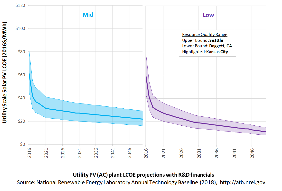
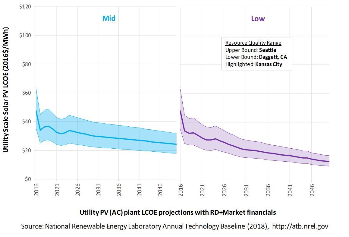
The following three figures illustrate LCOE, which includes the combined impact of CAPEX, O&M, and capacity factor projections for utility-scale PV across the range of resources present in the contiguous United States. For the purposes of the ATB, the costs associated with technology and project risk in the U.S. market are represented in the financing costs, not in the upfront capital costs (e.g. developer fees, contingencies). An individual technology may receive more favorable financing terms outside of the U.S., due to less technology and project risk, caused by more project development experience (e.g. offshore wind in Europe), or more government or market guarantees. The R&D Only LCOE sensitivity cases present the range of LCOE based on financial conditions that are held constant over time unless R&D affects them, and they reflect different levels of technology risk. This case excludes effects of tax reform, tax credits, technology-specific tariffs, and changing interest rates over time. The R&D + Market LCOE case adds to these the financial assumptions (1) the changes over time consistent with projections in the Annual Energy Outlook and (2) the effects of tax reform, tax credits, and tariffs. The ATB representative plant characteristics that best align with those of recently installed or anticipated near-term utility-scale PV plants are associated with Utility PV: Kansas City. Data for all the resource categories can be found in the ATB data spreadsheet.
R&D Only | R&D + Market
The methodology for representing the CAPEX, O&M, and capacity factor assumptions behind each pathway is discussed in Projections Methodology. In general, the degree of adoption of technology innovation distinguishes the Constant, Mid, and Low technology cost scenarios. These projections represent trends that reduce CAPEX and improve performance. Development of these scenarios involves technology-specific application of the following general definitions:
- Constant Technology Cost Scenario = Base Year (or near-term estimates of projects under construction) equivalent through 2050 maintains current relative technology cost differences
- Mid Technology Cost Scenario = technology advances through continued industry growth, public and private R&D investments, and market conditions relative to current levels that may be characterized as "likely" or "not surprising"
- Low Technology Cost Scenario = Technology advances that may occur with breakthroughs, increased public and private R&D investments, and/or other market conditions that lead to cost and performance levels that may be characterized as the " limit of surprise" but not necessarily the absolute low bound.
To estimate LCOE, assumptions about the cost of capital to finance electricity generation projects are required, and the LCOE calculations are sensitive to these financial assumptions. Three project finance structures are used within the ATB:
- R&D Only Financial Assumptions: This sensitivity case allows technology-specific changes to debt interest rates, return on equity rates, and debt fraction to reflect effects of R&D on technological risk perception, but it holds background rates constant at 2016 values from AEO 2018 and excludes effects of tax reform, tax credits, and tariffs.
- R&D Only + Market Financial Assumptions: This sensitivity case retains the technology-specific changes to debt interest, return on equity rates, and debt fraction from the R&D Only case and adds in the variation over time consistent with AEO 2018, as well as effects of tax reform, tax credits, and technology-specific tariffs. For a detailed discussion of these assumptions, see Changes from 2017 ATB to 2018 ATB.
- ReEDS Financial Assumptions: ReEDS uses the R&D Only + Market Financial Assumptions for the "Mid" technology cost scenario.
A constant cost recovery period -over which the initial capital investment is recovered-is assumed for all technologies throughout this website, and can be varied in the ATB data spreadsheet.
- The equations and variables used to estimate LCOE are defined on the equations and variables page. For illustration of the impact of changing financial structures such as WACC, see Project Finance Impact on LCOE. For LCOE estimates for the Constant, Mid, and Low technology cost scenarios for all technologies, see 2018 ATB Cost and Performance Summary.
In general, differences among the technology cost cases reflect different levels of adoption of innovations. Reductions in technology costs reflect the cost reduction opportunities that are listed below.
- Modules
- Increased module efficiencies and increased production-line throughput to decrease CAPEX; overhead costs on a per-kilowatt basis will go down if efficiency and throughput improvement are realized
- Reduced wafer thickness or the thickness of thin-film semiconductor layers
- Development of new semiconductor materials
- Development of larger manufacturing facilities in low-cost regions
- Balance of system (BOS)
- Increased module efficiency, reducing the size of the installation
- Development of racking systems that enhance energy production or require less robust engineering
- Integration of racking or mounting components in modules
- Reduction of supply chain complexity and cost
- Creation of standard packaged system design
- Improvement of supply chains for BOS components in modules
- Improved power electronics
- Improvement of inverter prices and performance, possibly by integrating microinverters
- Decreased installation costs and margins
- Reduction of supply chain margins (e.g., profit and overhead charged by suppliers, manufacturer, distributors, and retailers); this will likely occur naturally as the U.S. PV industry grows and matures
- Streamlining of installation practices through improved workforce development and training and developing standardized PV hardware
- Expansion of access to a range of innovative financing approaches and business models
- Development of best practices for permitting interconnection and PV installation such as subdivision regulations, new construction guidelines, and design requirements.
FOM cost reduction represents optimized O&M strategies, reduced component replacement costs, and lower frequency of component replacement.
References
Annual Energy Outlook 2017 with Projections to 2050. Washington, D.C.: U.S. Department of Energy. January 5, 2017. http://www.eia.gov/outlooks/aeo/pdf/0383(2017).pdf.
H2 2017 US PV Market Outlook. December 13, 2017. New York: BNEF.
Lazard's Levelized Cost of Energy Analysis: Version 11.0. November 2017. New York: Lazard. https://www.lazard.com/perspective/levelized-cost-of-energy-2017.
PV Market Outlook, Q4 2017. November 17, 2017. New York: BNEF.
ABB. 2017. Spring 2017 Power Reference Case: Preview of key changes & potential impacts. ABB Enterprise Software. April 5, 2017.
Bolinger, Mark, Joachim Seel, and Kristina Hamachi LaCommare. 2017. Utility-Scale Solar 2016: An Empirical Analysis of Project Cost, Performance, and Pricing Trends in the United States. Berkeley, CA: Lawrence Berkeley National Laboratory. LBNL- 2001055. September 2017. http://eta-publications.lbl.gov/sites/default/files/utility-scale_solar_2016_report.pdf.
Carlsson, J., M. del Mar Perez Fortes, G. de Marco, J. Giuntoli, M. Jakubcionis, A. Jäger-Waldau, R. Lacal-Arantegui, S. Lazarou, D. Magagna, C. Moles, B. Sigfusson, A. Spisto, M. Vallei, and E. Weidner. 2014. ETRI 2014: Energy Technology Reference Indicator, Projections for 2010-2050. European Commission: JRC Science and Policy Reports. http://publications.jrc.ec.europa.eu/repository/bitstream/JRC92496/ldna26950enn.pdf.
Denholm, P., and R. Margolis. 2008. "Land-Use Requirements and the Per-Capita Solar Footprint for Photovoltaic Generation in the United States." Energy Policy (36):3531–3543.
EIA (U.S. Energy Information Administration). 2016a. Capital Cost Estimates for Utility Scale Electricity Generating Plants. Washington, D.C.: U.S. Department of Energy. November 2016. https://www.eia.gov/analysis/studies/powerplants/capitalcost/pdf/capcost_assumption.pdf.
EIA (U.S. Energy Information Administration). 2018. Annual Energy Outlook 2018 with Projections to 2050. Washington, D.C.: U.S. Department of Energy. February 6, 2018. https://www.eia.gov/outlooks/aeo/pdf/AEO2018.pdf.
Feldman, David, Jack Hoskins, and Robert Margolis. 2017. Q2/Q3 2017 Solar Industry Update. U.S. Department of Energy. NREL/PR-6A42-70406. November 13, 2017. https://www.nrel.gov/docs/fy18osti/70406.pdf.
Fraunhofer ISE. 2015. Current and Future Cost of Photovoltaics: Long-term Scenarios for Market Development, System Prices and LCOE of Utility-Scale PV Systems. Prepared for Agora Energiewende. Freiburg, Germany: Fraunhofer-Institute for Solar Energy Systems (ISE). 059/01-S-2015/EN. February 2015. https://www.agora-energiewende.de/fileadmin/Projekte/2014/Kosten-Photovoltaik-2050/AgoraEnergiewende_Current_and_Future_Cost_of_PV_Feb2015_web.pdf.
Fu, Ran, David Feldman, Robert Margolis, Mike Woodhouse, and Kristen Ardani. 2017. U.S. Solar Photovoltaic System Cost Benchmark: Q1 2017. Golden, CO: National Renewable Energy Laboratory. NREL/TP-6A20-68925. https://www.nrel.gov/docs/fy17osti/68925.pdf.
GTM Research. 2016. U.S. PV System Pricing H1 2017: System Pricing, Breakdowns and Forecasts. Boston, MA: GTM Research. June 2017.
IEA (International Energy Agency). 2016. World Energy Outlook 2016. Paris: International Energy Agency. December 2016.
IHS. 2017. PV Demand Market Tracker. Q4 2017. IHS. December 8, 2017. https://technology.ihs.com/572649/pv-demand-market-tracker-q4-2017.
IRENA (International Renewable Energy Agency). n.d. "IRENA Renewable Cost Database." Accessed 2017: http://www.irena.org/costs.
Lopez, Anthony, Billy Roberts, Donna Heimiller, Nate Blair, and Gian Porro. 2012. U.S. Renewable Energy Technical Potentials: A GIS-Based Analysis. National Renewable Energy Laboratory. NREL/TP-6A20-51946. http://www.nrel.gov/docs/fy12osti/51946.pdf.
Teske, Sven, Steve Sawyer, and Oliver Schäfer, Thomas Pregger, Sonja Simon, and Tobias Naegler. 2015. Energy [r]evolution: A Sustainable World Energy Outlook 2015. Global Wind Energy Council, Solar Power Europe & Greenpeace. September 2015.